Optimization Algorithms in Neural Networks

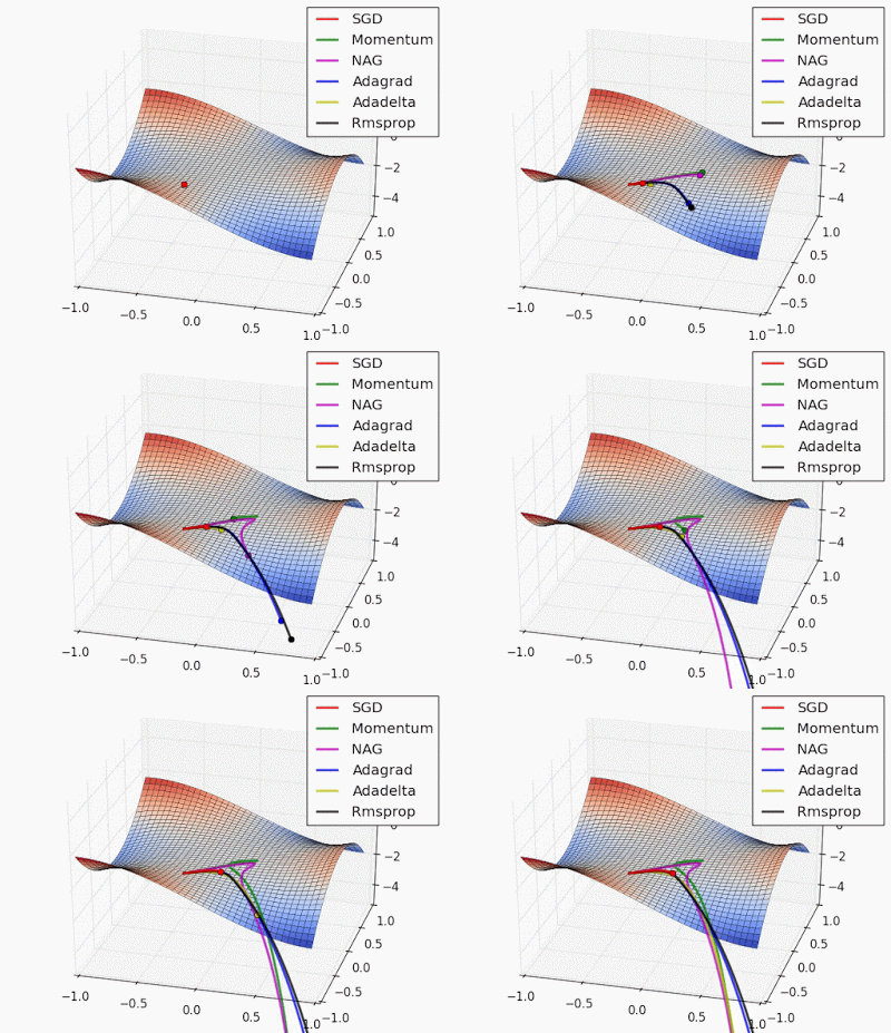
Overview of some of the most used optimizers while training a neural network.

Introduction

In deep learning, we have the concept of loss, which tells us how poorly the model is performing at that current instant. Now we need to use this loss to train our network such that it performs better. Essentially what we need to do is to take the loss and try to minimize it, because a lower loss means our model is going to perform better. The process of minimizing (or maximizing) any mathematical expression is called optimization.

Optimizers are algorithms or methods used to change the attributes of the neural network such as weights and learning rate to reduce the losses. Optimizers are used to solve optimization problems by minimizing the function.

How do Optimizers work?

For a useful mental model, you can think of a hiker trying to get down a mountain with a blindfold on. It’s impossible to know which direction to go in, but there’s one thing she can know: if she’s going down (making progress) or going up (losing progress). Eventually, if she keeps taking steps that lead her downwards, she’ll reach the base.

Similarly, it’s impossible to know what your model’s weights should be right from the start. But with some trial and error based on the loss function (whether the hiker is descending), you can end up getting there eventually.

How you should change your weights or learning rates of your neural network to reduce the losses is defined by the optimizers you use. Optimization algorithms are responsible for reducing the losses and to provide the most accurate results possible.

Various optimizers are researched within the last few couples of years each having its advantages and disadvantages. Read the entire article to understand the working, advantages, and disadvantages of the algorithms.

We’ll learn about different types of optimizers and how they exactly work to minimize the loss function.

1. Gradient Descent
2. Stochastic Gradient Descent (SGD)
3. Mini Batch Stochastic Gradient Descent (MB-SGD)
4. SGD with momentum
5. Nesterov Accelerated Gradient (NAG)
6. Adaptive Gradient (AdaGrad)
7. AdaDelta
8. RMSprop
9. Adam

Gradient Descent

Gradient descent is an optimization algorithm that’s used when training a machine learning model. It’s based on a convex function and tweaks its parameters iteratively to minimize a given function to its local minimum.

WHAT IS GRADIENT DESCENT? Gradient Descent is an optimization algorithm for finding a local minimum of a differentiable function. Gradient descent is simply used to find the values of a function’s parameters (coefficients) that minimize a cost function as far as possible.

You start by defining the initial parameter’s values and from there gradient descent uses calculus to iteratively adjust the values so they minimize the given cost-function.

The weight is initialized using some initialization strategies and is updated with each epoch according to the update equation.

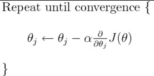
The above equation computes the gradient of the cost function J(θ) w.r.t. to the parameters/weights θ for the entire training dataset:

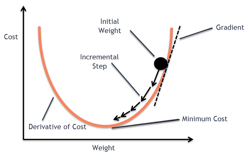
Our aim is to get to the bottom of our graph(Cost vs weights), or to a point where we can no longer move downhill–a local minimum.

Okay now, what is Gradient?

“A gradient measures how much the output of a function changes if you change the inputs a little bit.” — Lex Fridman (MIT)

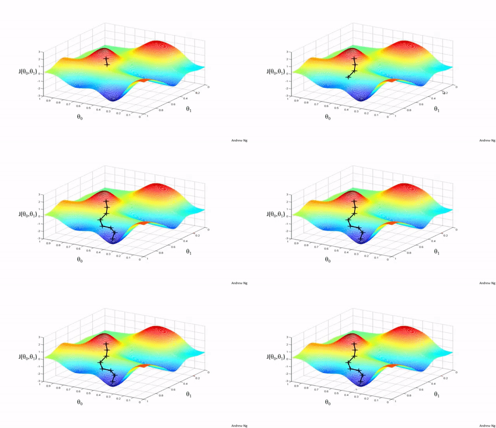
Importance of Learning rate

How big the steps are gradient descent takes into the direction of the local minimum are determined by the learning rate, which figures out how fast or slows we will move towards the optimal weights.

For gradient descent to reach the local minimum we must set the learning rate to an appropriate value, which is neither too low nor too high. This is important because if the steps it takes are too big, it may not reach the local minimum because it bounces back and forth between the convex function of gradient descent (see left image below). If we set the learning rate to a very small value, gradient descent will eventually reach the local minimum but that may take a while (see the right image).

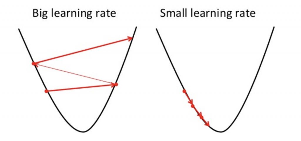
So, the learning rate should never be too high or too low for this reason. You can check if you’re learning rate is doing well by plotting it on a graph.

In code, gradient descent looks something like this:

for i in range(nb_epochs):   
    params_grad = evaluate_gradient(loss_function, data, params)           
    params = params - learning_rate * params_grad

For a pre-defined number of epochs, we first compute the gradient vector params_grad of the loss function for the whole dataset w.r.t. our parameter vector params.

Advantages:

1. Easy computation.
2. Easy to implement.
3. Easy to understand.

Disadvantages:

1. May trap at local minima.
2. Weights are changed after calculating the gradient on the whole dataset. So, if the dataset is too large then this may take years to converge to the minima.
3. Requires large memory to calculate the gradient on the whole dataset.

Stochastic Gradient Descent (SGD)

SGD algorithm is an extension of the Gradient Descent and it overcomes some of the disadvantages of the GD algorithm. Gradient Descent has a disadvantage that it requires a lot of memory to load the entire dataset of n-points at a time to compute the derivative of the loss function. In the SGD algorithm derivative is computed taking one point at a time.

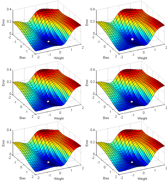
SGD performs a parameter update for each training example x(i) and label y(i):

θ = θ − α⋅∂(J(θ;x(i),y(i)))/∂θ

where {x(i) ,y(i)} are the training examples.

To make the training even faster we take a Gradient Descent step for each training example. Let’s see what the implications would be in the image below.

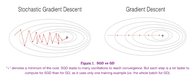
1. On the left, we have Stochastic Gradient Descent (where m=1 per step) we take a Gradient Descent step for each example and on the right is Gradient Descent (1 step per entire training set).
2. SGD seems to be quite noisy, at the same time it is much faster but may not converge to a minimum.
3. Typically, to get the best out of both worlds we use Mini-batch gradient descent (MGD) which looks at a smaller number of training set examples at once to help (usually power of 2 – 2^6 etc.).
4. Mini-batch Gradient Descent is relatively more stable than Stochastic Gradient Descent (SGD) but does have oscillations as gradient steps are being taken in the direction of a sample of the training set and not the entire set as in BGD.

It is observed that in SGD the updates take more number iterations compared to gradient descent to reach minima. On the right, the Gradient Descent takes fewer steps to reach minima but the SGD algorithm is noisier and takes more iterations.

Its code fragment simply adds a loop over the training examples and evaluates the gradient w.r.t. each example.

for i in range(nb_epochs):
    np.random.shuffle(data)
    for example in data:
        params_grad = evaluate_gradient(loss_function, example, params)
        params = params - learning_rate * params_grad

Advantage:

Memory requirement is less compared to the GD algorithm as the derivative is computed taking only 1 point at once.

Disadvantages:

1. The time required to complete 1 epoch is large compared to the GD algorithm.
2. Takes a long time to converge.
3. May stuck at local minima.

Mini Batch Stochastic Gradient Descent (MB-SGD)

MB-SGD algorithm is an extension of the SGD algorithm and it overcomes the problem of large time complexity in the case of the SGD algorithm. MB-SGD algorithm takes a batch of points or subset of points from the dataset to compute derivate.

It is observed that the derivative of the loss function for MB-SGD is almost the same as a derivate of the loss function for GD after some number of iterations. But the number of iterations to achieve minima is large for MB-SGD compared to GD and the cost of computation is also large.

The update of weight is dependent on the derivate of loss for a batch of points. The updates in the case of MB-SGD are much noisy because the derivative is not always towards minima.

MB-SGD divides the dataset into various batches and after every batch, the parameters are updated.

θ = θ − α⋅∂(J(θ;B(i)))/∂θ

where {B(i)} are the batches of training examples.

In code, instead of iterating over examples, we now iterate over mini-batches of size 50:

for i in range(nb_epochs):
    np.random.shuffle(data)
    for batch in get_batches(data, batch_size=50):
        params_grad = evaluate_gradient(loss_function, batch, params)
        params = params - learning_rate * params_grad

Advantages:

Less time complexity to converge compared to standard SGD algorithm.

Disadvantages:

1. The update of MB-SGD is much noisy compared to the update of the GD algorithm.
2. Take a longer time to converge than the GD algorithm.
3. May get stuck at local minima.

SGD with momentum

A major disadvantage of the MB-SGD algorithm is that updates of weight are very noisy. SGD with momentum overcomes this disadvantage by denoising the gradients. Updates of weight are dependent on noisy derivative and if we somehow denoise the derivatives then converging time will decrease.

The idea is to denoise derivative using exponential weighting average that is to give more weightage to recent updates compared to the previous update.

It accelerates the convergence towards the relevant direction and reduces the fluctuation to the irrelevant direction. One more hyperparameter is used in this method known as momentum symbolized by ‘γ’.

V(t)= γ.V(t−1)+ α.∂(J(θ))/∂θ

Now, the weights are updated by θ = θ − V(t).

The momentum term γ is usually set to 0.9 or a similar value.

Momentum at time ‘t’ is computed using all previous updates giving more weightage to recent updates compared to the previous update. This leads to speed up the convergence.

Essentially, when using momentum, we push a ball down a hill. The ball accumulates momentum as it rolls downhill, becoming faster and faster on the way (until it reaches its terminal velocity if there is air resistance, i.e. γ<1). The same thing happens to our parameter updates: The momentum term increases for dimensions whose gradients point in the same directions and reduces updates for dimensions whose gradients change directions. As a result, we gain faster convergence and reduced oscillation.

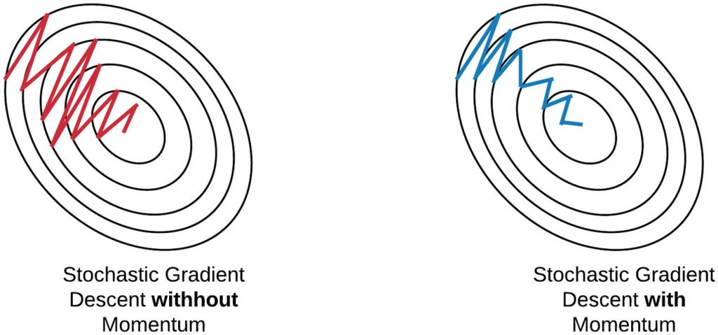
The diagram above concludes SGD with momentum denoises the gradients and converges faster as compared to SGD.

Advantages:

1. Has all advantages of the SGD algorithm.
2. Converges faster than the GD algorithm.

Disadvantages:

We need to compute one more variable for each update.

Nesterov Accelerated Gradient (NAG)

The idea of the NAG algorithm is very similar to SGD with momentum with a slight variant. In the case of SGD with a momentum algorithm, the momentum and gradient are computed on the previous updated weight.

Momentum may be a good method but if the momentum is too high the algorithm may miss the local minima and may continue to rise up. So, to resolve this issue the NAG algorithm was developed. It is a look ahead method. We know we’ll be using γ.V(t−1) for modifying the weights so, θ−γV(t−1) approximately tells us the future location. Now, we’ll calculate the cost based on this future parameter rather than the current one.

V(t)= γ.V(t−1)+ α.∂(J(θ − γV(t−1)))/∂θ

and then update the parameters using θ = θ − V(t)

Again, we set the momentum term γγ to a value of around 0.9. While Momentum first computes the current gradient (small brown vector in Image 4) and then takes a big jump in the direction of the updated accumulated gradient (big brown vector), NAG first makes a big jump in the direction of the previously accumulated gradient (green vector), measures the gradient and then makes a correction (red vector), which results in the complete NAG update (red vector). This anticipatory update prevents us from going too fast and results in increased responsiveness, which has significantly increased the performance of RNNs on a number of tasks.

Both NAG and SGD with momentum algorithms work equally well and share the same advantages and disadvantages.

Adaptive Gradient Descent(AdaGrad)

For all the previously discussed algorithms the learning rate remains constant. So the key idea of AdaGrad is to have an adaptive learning rate for each of the weights.

It performs smaller updates for parameters associated with frequently occurring features, and larger updates for parameters associated with infrequently occurring features.

For brevity, we use gt to denote the gradient at time step t. gt,i is then the partial derivative of the objective function w.r.t. to the parameter θi at time step t, η isthe learning rate and ∇θ is the partial derivative of loss function J(θi)

In its update rule, Adagrad modifies the general learning rate η at each time step t for every parameter θi based on the past gradients for θi:

where Gt is the sum of the squares of the past gradients w.r.t to all parameters θ.

The benefit of AdaGrad is that it eliminates the need to manually tune the learning rate; most leave it at a default value of 0.01.

Its main weakness is the accumulation of the squared gradients(Gt) in the denominator. Since every added term is positive, the accumulated sum keeps growing during training, causing the learning rate to shrink and becoming infinitesimally small and further resulting in a vanishing gradient problem.

Advantage:

No need to update the learning rate manually as it changes adaptively with iterations.

Disadvantage:

As the number of iteration becomes very large learning rate decreases to a very small number which leads to slow convergence.

AdaDelta

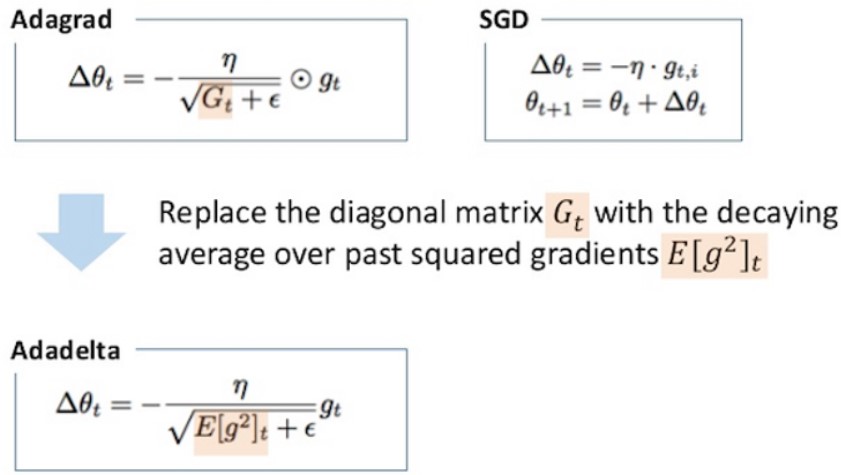
The problem with the previous algorithm AdaGrad was learning rate becomes very small with a large number of iterations which leads to slow convergence. To avoid this, the AdaDelta algorithm has an idea to take an exponentially decaying average.

Adadelta is a more robust extension of Adagrad that adapts learning rates based on a moving window of gradient updates, instead of accumulating all past gradients. This way, Adadelta continues learning even when many updates have been done. Compared to Adagrad, in the original version of Adadelta, you don’t have to set an initial learning rate.

Instead of inefficiently storing w previous squared gradients, the sum of gradients is recursively defined as a decaying average of all past squared gradients. The running average E[g2]t at time step t then depends only on the previous average and current gradient:

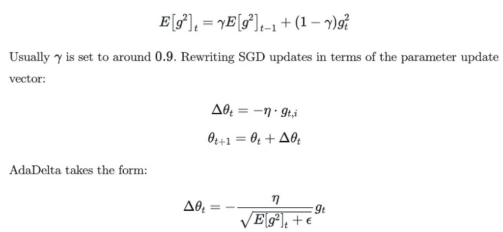
With Adadelta, we do not even need to set a default learning rate, as it has been eliminated from the update rule.

RMSprop

RMSprop in fact is identical to the first update vector of Adadelta that we derived above:

RMSprop as well divides the learning rate by an exponentially decaying average of squared gradients. Hinton suggests γ be set to 0.9, while a good default value for the learning rate η is 0.001.

RMSprop and Adadelta have both been developed independently around the same time stemming from the need to resolve Adagrad’s radically diminishing learning rates

Adaptive Moment Estimation (Adam)

Adam can be looked at as a combination of RMSprop and Stochastic Gradient Descent with momentum.

Adam computes adaptive learning rates for each parameter. In addition to storing an exponentially decaying average of past squared gradients vt like Adadelta and RMSprop, Adam also keeps an exponentially decaying average of past gradients mt, similar to momentum. Whereas momentum can be seen as a ball running down a slope, Adam behaves like a heavy ball with friction, which thus prefers flat minima in the error surface.

Hyper-parameters β1, β2 ∈ [0, 1) control the exponential decay rates of these moving averages. We compute the decaying averages of past and past squared gradients mt and vt respectively as follows:

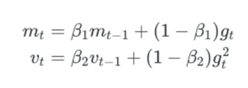
mt and vt are estimates of the first moment (the mean) and the second moment (the uncentered variance) of the gradients respectively, hence the name of the method.

When to choose which algorithm?

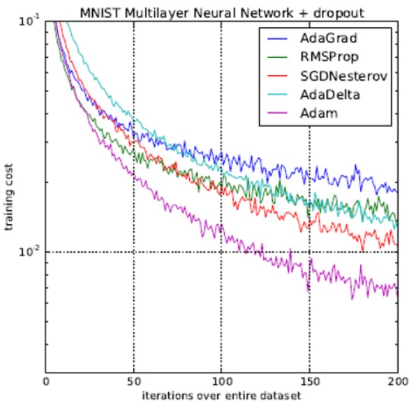
As you can observe, the training cost in the case of Adam is the least.

Now observe the animation at the beginning of this article and consider the following points:

1. It is observed that the SGD algorithm (red) is stuck at a saddle point. So SGD algorithm can only be used for shallow networks.
2. All the other algorithms except SGD finally converges one after the other, AdaDelta being the fastest followed by momentum algorithms.
3. AdaGrad and AdaDelta algorithm can be used for sparse data.
4. Momentum and NAG work well for most cases but is slower.
5. Animation for Adam is not available but from the plot above it is observed that it is the fastest algorithm to converge to minima.
6. Adam is considered the best algorithm amongst all the algorithms discussed above.

To understand how to implement all these optimization algorithms in neural networks using python you can have a look here.

Note: This article was originally published on theaidream, and kindly contributed to AI Planet (formerly DPhi) to spread the knowledge.

References:

https://towardsdatascience.com/overview-of-various-optimizers-in-neural-networks-17c1be2df6d5

https://towardsdatascience.com/optimizers-for-training-neural-network-59450d71caf6

https://towardsdatascience.com/stochastic-gradient-descent-with-momentum-a84097641a5d

https://ruder.io/optimizing-gradient-descent/