Introduction

The simplest solutions are usually the most powerful ones, and Naïve Bayes is a good example of that. Despite the advances in Machine Learning in the last years, it has proven to not only be simple but also fast, accurate, and reliable. It has been successfully used for many purposes, but it works particularly well with natural language processing (NLP) problems.

Naïve Bayes is a probabilistic machine learning algorithm based on the Bayes Theorem, used in a wide variety of classification tasks. In this article, we will understand the Naïve Bayes algorithm and all essential concepts so that there is no room for doubts in understanding.

Bayes Theorem

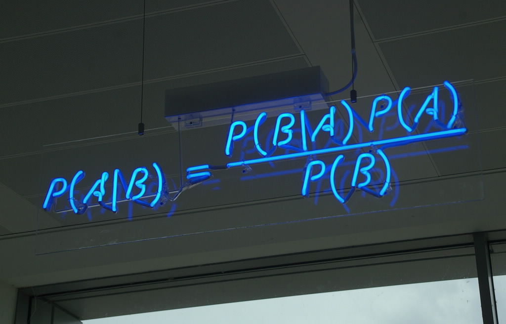
Bayes’ Theorem is a simple mathematical formula used for calculating conditional probabilities.

Conditional probability is a measure of the probability of an event occurring given that another event has (by assumption, presumption, assertion, or evidence) occurred.

The formula is: —

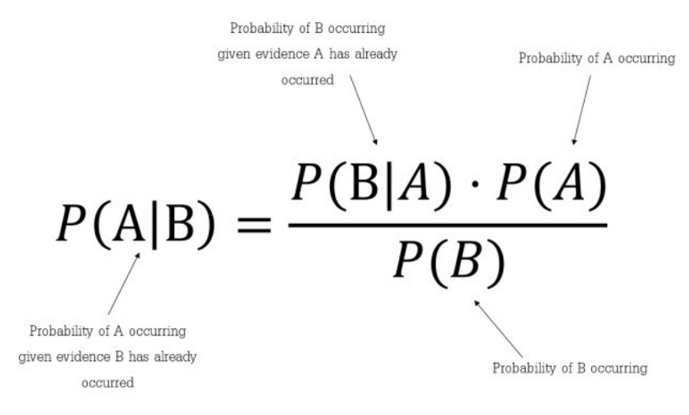
Which tells us: how often A happens given that B happens, written P(A|B) also called posterior probability, When we know: how often B happens given that A happens, written P(B|A) and how likely A is on its own, written P(A) and how likely B is on its own, written P(B).

In simpler terms, Bayes’ Theorem is a way of finding a probability when we know certain other probabilities.

Assumptions made by Naïve Bayes

The fundamental Naïve Bayes assumption is that each feature makes an:

• independent
• equal

contribution to the outcome.

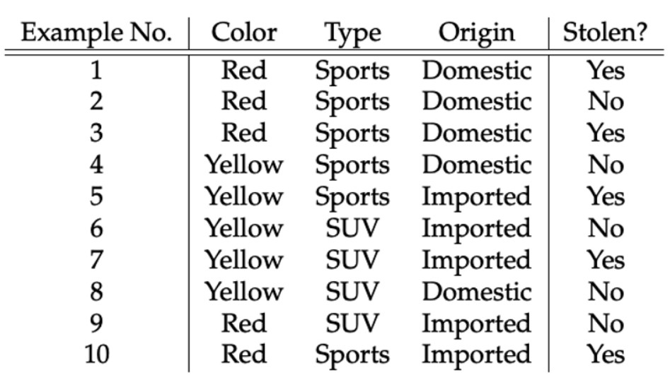
Let us take an example to get some better intuition. Consider the car theft problem with attributes Color, Type, Origin, and the target, Stolen can be either Yes or No.

Example

The dataset is represented as below.

Concerning our dataset, the concept of assumptions made by the algorithm can be understood as:

• We assume that no pair of features are dependent. For example, the color being ‘Red’ has nothing to do with the Type or the Origin of the car. Hence, the features are assumed to be Independent.
• Secondly, each feature is given the same influence(or importance). For example, knowing the only Color and Type alone can’t predict the outcome perfectly. So none of the attributes are irrelevant and assumed to be contributing Equally to the outcome.

Note: The assumptions made by Naïve Bayes are generally not correct in real-world situations. The independence assumption is never correct but often works well in practice. Hence the name ‘Naïve’.

Here in our dataset, we need to classify whether the car is stolen, given the features of the car.

The columns represent these features and the rows represent individual entries. If we take the first row of the dataset, we can observe that the car is stolen if the Color is Red, the Type is Sports and the Origin is Domestic. So we want to classify a Red Domestic SUV is getting stolen or not. Note that there is no example of a Red Domestic SUV in our data set.

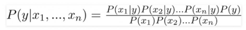
According to this example, Bayes theorem can be rewritten as:

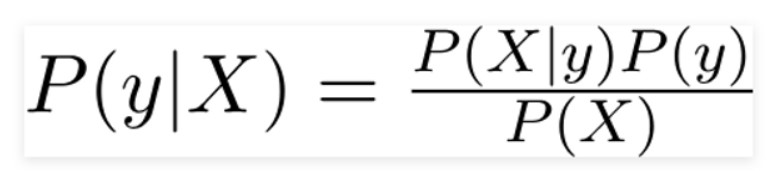
The variable y is the class variable(stolen?), which represents if the car is stolen or not given the conditions. Variable X represents the parameters/features.

X is given as,

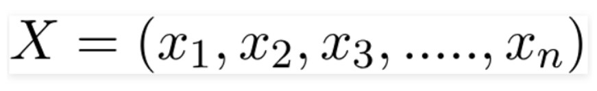
Here x1,x2….xn represent the features, i.e they can be mapped to Color, Type, and Origin. By substituting for X and expanding using the chain rule we get,

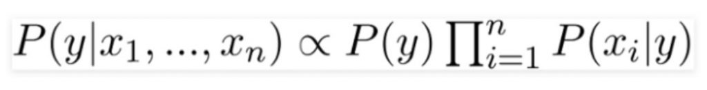
Now, you can obtain the values for each by looking at the dataset and substitute them into the equation. For all entries in the dataset, the denominator does not change, it remains static. Therefore, the denominator can be removed and proportionality can be injected.

In our case, the class variable(y) has only two outcomes, yes or no. There could be cases where the classification could be multivariate. Therefore, we have to find the class variable(y) with maximum probability.

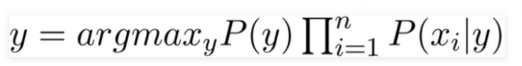
Using the above function, we can obtain the class, given the predictors/features.

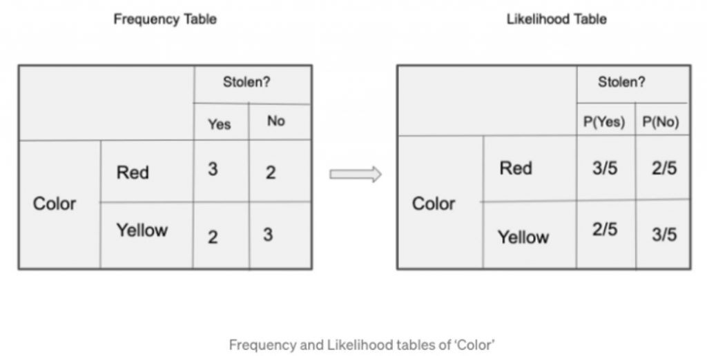
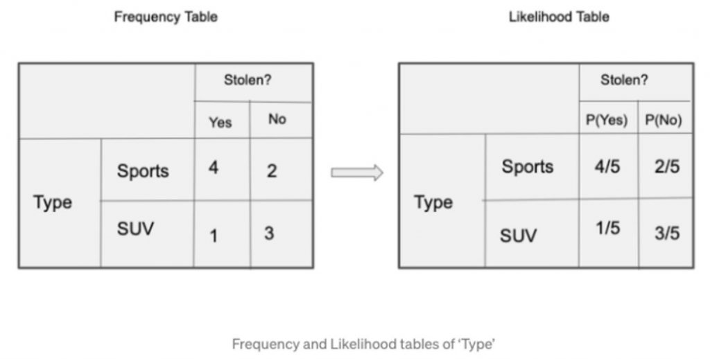
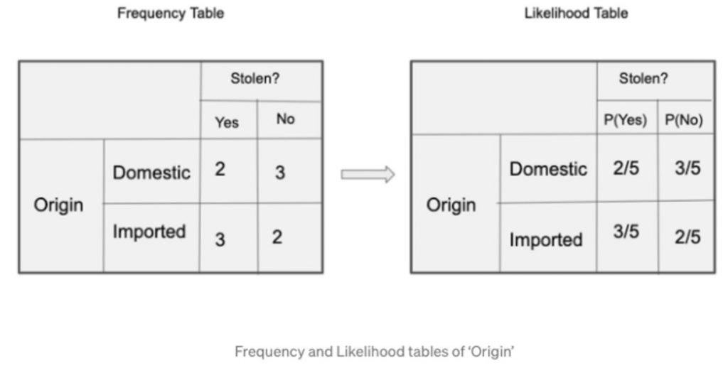
The posterior probability P(y|X) can be calculated by first, creating a Frequency Table for each attribute against the target. Then, molding the frequency tables to Likelihood Tables and finally, use the Naïve Bayesian equation to calculate the posterior probability for each class. The class with the highest posterior probability is the outcome of the prediction. Below are the Frequency and likelihood tables for all three predictors.

So in our example, we have 3 predictors X.

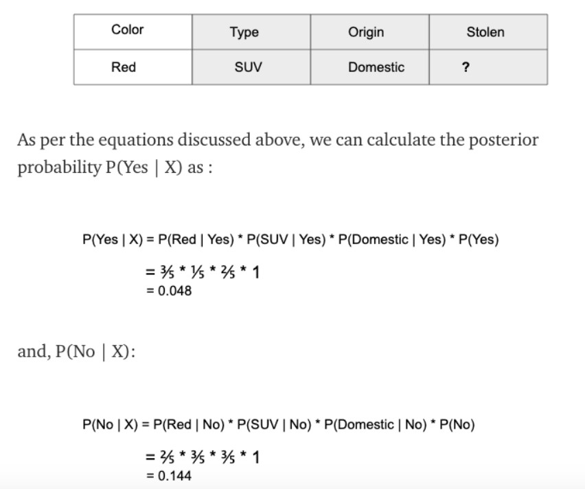
Since 0.144 > 0.048, Which means given the features RED SUV and Domestic, our example gets classified as ’NO’ the car is not stolen.

The zero-frequency problem

One of the disadvantages of Naïve-Bayes is that if you have no occurrences of a class label and a certain attribute value together then the frequency-based probability estimate will be zero. And this will get a zero when all the probabilities are multiplied.

An approach to overcome this ‘zero-frequency problem’ in a Bayesian environment is to add one to the count for every attribute value-class combination when an attribute value doesn’t occur with every class value.

For example, say your training data looked like this:

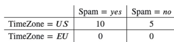
𝑃(TimeZone=𝑈𝑆|Spam=𝑦𝑒𝑠)=10/10=1

𝑃(TimeZone=𝐸𝑈|Spam=𝑦𝑒𝑠)=0/10=0

Then you should add one to every value in this table when you’re using it to calculate probabilities:

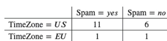
𝑃(TimeZone=𝑈𝑆|Spam=𝑦𝑒𝑠)=11/12

𝑃(TimeZone=𝐸𝑈|Spam=𝑦𝑒𝑠)=1/12

This is how we’ll get rid of getting a zero probability.

Types of Naïve Bayes Classifier:

• Multinomial Naïve Bayes: Feature vectors represent the frequencies with which certain events have been generated by a multinomial distribution. This is the event model typically used for document classification.
• Bernoulli Naïve Bayes: In the multivariate Bernoulli event model, features are independent booleans (binary variables) describing inputs. Like the multinomial model, this model is popular for document classification tasks, where binary term occurrence(i.e. a word occurs in a document or not) features are used rather than term frequencies(i.e. frequency of a word in the document).
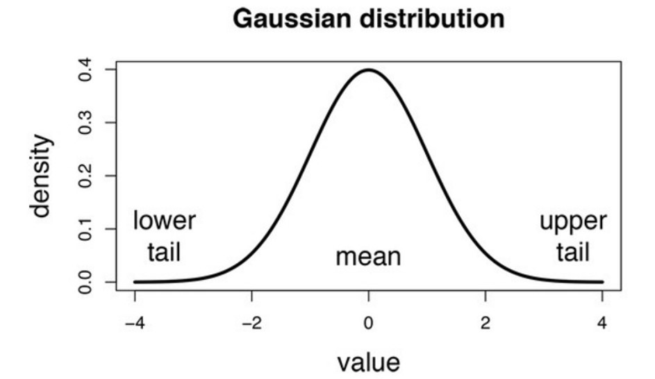
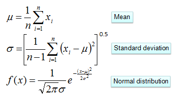
• Gaussian Naïve Bayes: In Gaussian Naïve Bayes, continuous values associated with each feature are assumed to be distributed according to a Gaussian distribution(Normal distribution). When plotted, it gives a bell-shaped curve which is symmetric about the mean of the feature values as shown below:

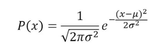
The likelihood of the features is assumed to be Gaussian, hence, conditional probability is given by:

Now, what if any feature contains numerical values instead of categories i.e. Gaussian distribution.

One option is to transform the numerical values to their categorical counterparts before creating their frequency tables. The other option, as shown above, could be using the distribution of the numerical variable to have a good guess of the frequency. For example, one common method is to assume normal or gaussian distributions for numerical variables.

The probability density function for the normal distribution is defined by two parameters (mean and standard deviation).

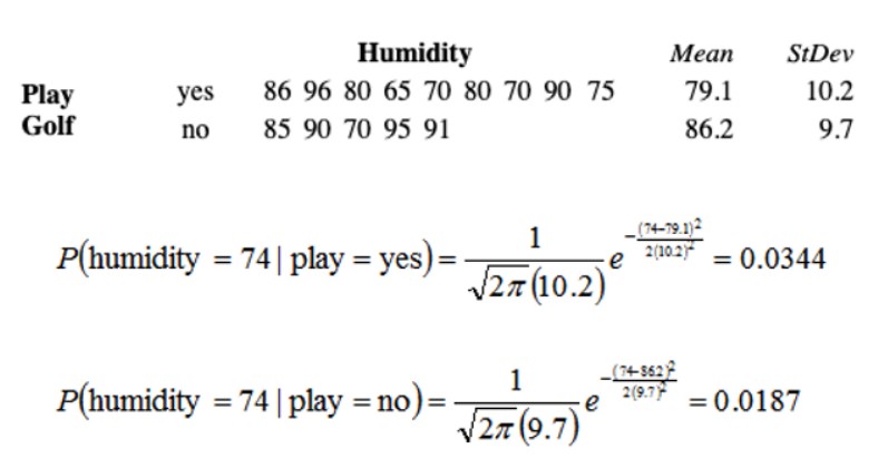
Consider the problem of playing golf, here the only predictor is Humidity, and Play Golf? is the target. Using the above formula we can calculate posterior probability if we know the mean and standard deviation.

Case study: Naïve Bayes classifier from scratch using Python

An existing problem for any major website today is how to handle virulent and divisive content. Quora wants to tackle this problem to keep its platform a place where users can feel safe sharing their knowledge with the world.

Quora is a platform that empowers people to learn from each other. On Quora, people can ask questions and connect with others who contribute unique insights and quality answers. A key challenge is to weed out insincere questions — those founded upon false premises, or that intend to make a statement rather than look for helpful answers.

The goal is to develop a Naïve Bayes classification model that identifies and flags insincere questions.

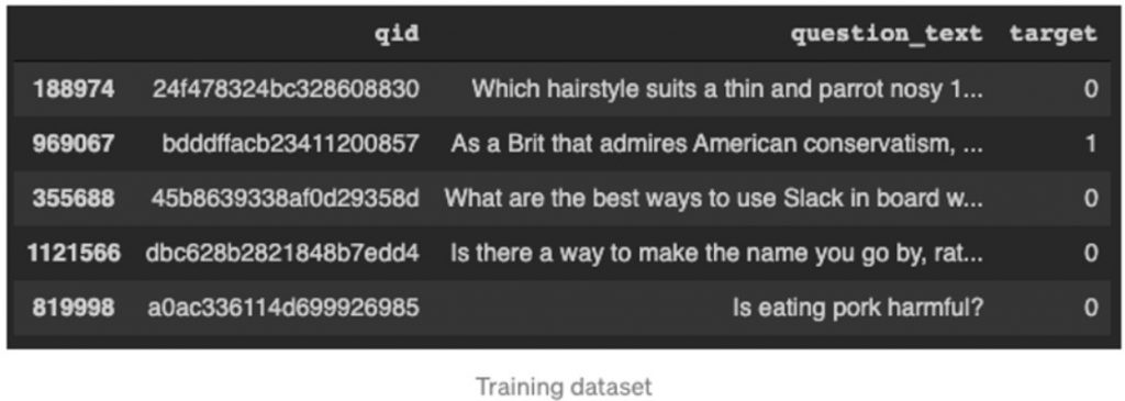
The dataset can be downloaded from here. Once you have downloaded the train and test data, load it and check.

import numpy as np
import pandas as pd
import os
train = pd.read_csv('./drive/My Drive/train.csv')
print(train.head())test = pd.read_csv('./drive/My Drive/test.csv')

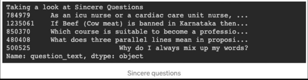
Let us see how are sincere questions look like.

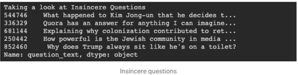
we see how are insincere questions look like.

Text Preprocessing:

The next step is to preprocess text before splitting the dataset into a train and test set. The preprocessing steps involve: Removing Numbers, Removing Punctuations in a string, Removing Stop Words, Stemming of Words, and Lemmatization of Words.

Constructing a Naive Bayes Classifier:

Combine all the preprocessing techniques and create a dictionary of words and each word’s count in training data.

1. Calculate probability for each word in a text and filter the words which have a probability less than threshold probability. Words with probability less than threshold probability are irrelevant.
2. Then for each word in the dictionary, create a probability of that word being in insincere questions and its probability insincere questions. Then finding the conditional probability to use in naive Bayes classifier.
3. Prediction using conditional probabilities.

You can checkout python code in this repository: https://gist.github.com/nageshsinghc4/4c9334815f904b1b6857e8d610c1e92d

Conclusion

Naïve Bayes algorithms are often used in sentiment analysis, spam filtering, recommendation systems, etc. They are quick and easy to implement but their biggest disadvantage is that the requirement of predictors to be independent.

Thanks for Reading!!!

Note: This article was originally published on theaidream, and kindly contributed to AI Planet (formerly DPhi) to spread the knowledge.