Audio Data Analysis Using Deep Learning with Python (Part 1)

A brief introduction to audio data processing and genre classification using Neural Networks and python.

Introduction

While much of the literature and buzz on deep learning concerns computer vision and natural language processing(NLP), audio analysis — a field that includes automatic speech recognition(ASR), digital signal processing, and music classification, tagging, and generation — is a growing subdomain of deep learning applications. Some of the most popular and widespread machine learning systems, virtual assistants Alexa, Siri, and Google Home, are largely products built atop models that can extract information from audio signals.

Audio data analysis is about analyzing and understanding audio signals captured by digital devices, with numerous applications in the enterprise, healthcare, productivity, and smart cities. Applications include customer satisfaction analysis from customer support calls, media content analysis and retrieval, medical diagnostic aids and patient monitoring, assistive technologies for people with hearing impairments, and audio analysis for public safety.

In the first part of this article series, we will talk about all you need to know before getting started with the audio data analysis and extract necessary features from a sound/audio file. We will also build an Artificial Neural Network(ANN) for the music genre classification. In the second part, we will accomplish the same by creating the Convolutional Neural Network and will compare their accuracy.

Table of Contents

• Audio file overview
• Applications of Audio Processing
• Audio Processing with Python
• Spectrogram
• Feature extraction from Audio signal
• Genre classification using Artificial Neural Networks(ANN).

Audio file overview

The sound excerpts are digital audio files in .wav format. Sound waves are digitized by sampling them at discrete intervals known as the sampling rate (typically 44.1kHz for CD-quality audio meaning samples are taken 44,100 times per second).

Each sample is the amplitude of the wave at a particular time interval, where the bit depth determines how detailed the sample will be also known as the dynamic range of the signal (typically 16bit which means a sample can range from 65,536 amplitude values).

What is Sampling and Sampling frequency? In signal processing, sampling is the reduction of a continuous signal into a series of discrete values. The sampling frequency or rate is the number of samples taken over some fixed amount of time. A high sampling frequency results in less information loss but higher computational expense, and low sampling frequencies have higher information loss but are fast and cheap to compute.

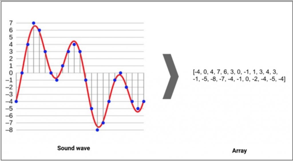
A sound wave, in red, represented digitally, in blue (after sampling and 4-bit quantization), with the resulting array shown on the right. Original © Aquegg | Wikimedia Commons

Applications of Audio Processing

What are the potential applications of audio processing? Here I would list a few of them:

• Indexing music collections according to their audio features.
• Recommending music for radio channels
• Similarity search for audio files (aka Shazam)
• Speech processing and synthesis — generating artificial voice for conversational agents

Audio Data Handling using Python

Sound is represented in the form of an audio signal having parameters such as frequency, bandwidth, decibel, etc. A typical audio signal can be expressed as a function of Amplitude and Time.

Frequency vs Time

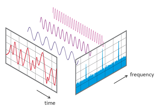
There are devices built that help you catch these sounds and represent it in a computer-readable format. Examples of these formats are

• wav (Waveform Audio File) format
• mp3 (MPEG-1 Audio Layer 3) format
• WMA (Windows Media Audio) format

A typical audio processing process involves the extraction of acoustics features relevant to the task at hand, followed by decision-making schemes that involve detection, classification, and knowledge fusion. Thankfully we have some useful python libraries which make this task easier.

Python Audio Libraries:

Python has some great libraries for audio processing like Librosa and PyAudio.There are also built-in modules for some basic audio functionalities.

We will mainly use two libraries for audio acquisition and playback:

1. Librosa

It is a Python module to analyze audio signals in general but geared more towards music. It includes the nuts and bolts to build a MIR(Music information retrieval) system. It has been very well documented along with a lot of examples and tutorials.

Installation:

pip install librosa
or
conda install -c conda-forge librosa

To fuel more audio-decoding power, you can install ffmpeg which ships with many audio decoders.

2. IPython.display.Audio

IPython.display.Audio lets you play audio directly in a jupyter notebook.

I have uploaded a random audio file on the below page. Let us now load the file in your jupyter console.

https://vocaroo.com/iMPozIbzB8T

Loading an audio file:

import librosa
audio_data = '/../../gruesome.wav'
x , sr = librosa.load(audio_data)
print(type(x), type(sr))#<class 'numpy.ndarray'> <class 'int'>print(x.shape, sr)#(94316,) 22050

This returns an audio time series as a numpy array with a default sampling rate(sr) of 22KHZ mono. We can change this behavior by resampling at 44.1KHz.

librosa.load(audio_data, sr=44100)

, or to disable resampling.

librosa.load(audio_path, sr=None)

The sample rate is the number of samples of audio carried per second, measured in Hz or kHz.

Playing Audio:

Using,IPython.display.Audio you can play the audio in your jupyter notebook.

import IPython.display as ipd
ipd.Audio(audio_data)

This returns an audio widget:

Visualizing Audio:

We can plot the audio array using librosa.display.waveplot:

%matplotlib inline
import matplotlib.pyplot as plt
import librosa.display
plt.figure(figsize=(14, 5))
librosa.display.waveplot(x, sr=sr)

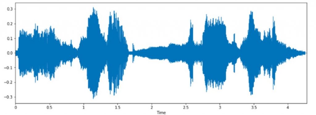
Here, we have the plot of the amplitude envelope of a waveform.

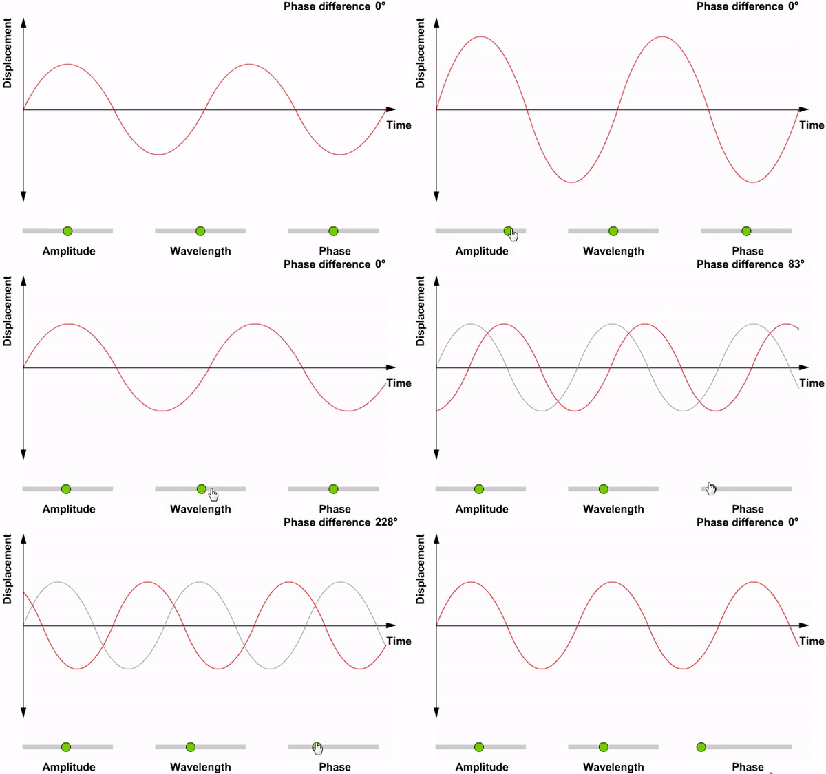
What is Amplitude, Wavelength, and Phase in a signal?

Spectrogram

A spectrogram is a visual way of representing the signal strength, or “loudness”, of a signal over time at various frequencies present in a particular waveform. Not only can one see whether there is more or less energy at, for example, 2 Hz vs 10 Hz, but one can also see how energy levels vary over time.

A spectrogram is usually depicted as a heat map, i.e., as an image with the intensity shown by varying the color or brightness.

We can display a spectrogram using. librosa.display.specshow.

X = librosa.stft(x)
Xdb = librosa.amplitude_to_db(abs(X))
plt.figure(figsize=(14, 5))
librosa.display.specshow(Xdb, sr=sr, x_axis='time', y_axis='hz')
plt.colorbar()

.stft() converts data into short term Fourier transform. STFT converts signals such that we can know the amplitude of the given frequency at a given time. Using STFT we can determine the amplitude of various frequencies playing at a given time of an audio signal. .specshow is used to display a spectrogram.

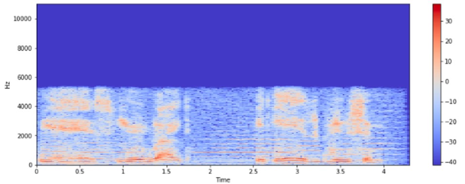
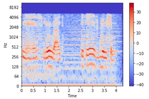
The vertical axis shows frequencies (from 0 to 10kHz), and the horizontal axis shows the time of the clip. Since we see that all action is taking place at the bottom of the spectrum, we can convert the frequency axis to a logarithmic one.

librosa.display.specshow(Xdb, sr=sr, x_axis='time', y_axis='log')
plt.colorbar()

Create an Audio Signal:

import numpy as np
sr = 22050 # sample rate
T = 5.0    # seconds
t = np.linspace(0, T, int(T*sr), endpoint=False) # time variable
x = 0.5*np.sin(2*np.pi*220*t)# pure sine wave at 220 Hz
#Playing the audio
ipd.Audio(x, rate=sr) # load a NumPy array
#Saving the audio
librosa.output.write_wav('tone_220.wav', x, sr)

Feature extraction from Audio signal

Every audio signal consists of many features. However, we must extract the characteristics that are relevant to the problem we are trying to solve. The process of extracting features to use them for analysis is called feature extraction. Let us study a few of the features in detail.

The spectral features (frequency-based features), which are obtained by converting the time-based signal into the frequency domain using the Fourier Transform, like fundamental frequency, frequency components, spectral centroid, spectral flux, spectral density, spectral roll-off, etc.

1. Spectral Centroid

The spectral centroid indicates at which frequency the energy of a spectrum is centered upon or in other words It indicates where the ” center of mass” for a sound is located. This is like a weighted mean:

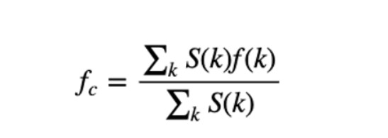
where S(k) is the spectral magnitude at frequency bin k, f(k) is the frequency at bin k.

librosa.feature.spectral_centroid computes the spectral centroid for each frame in a signal:

import sklearn
spectral_centroids = librosa.feature.spectral_centroid(x, sr=sr)[0]
spectral_centroids.shape
(775,)
# Computing the time variable for visualization
plt.figure(figsize=(12, 4))frames = range(len(spectral_centroids))
t = librosa.frames_to_time(frames)
# Normalising the spectral centroid for visualisation
def normalize(x, axis=0):
    return sklearn.preprocessing.minmax_scale(x, axis=axis)
#Plotting the Spectral Centroid along the waveform
librosa.display.waveplot(x, sr=sr, alpha=0.4)
plt.plot(t, normalize(spectral_centroids), color='b')

.spectral_centroid will return an array with columns equal to the number of frames present in your sample.

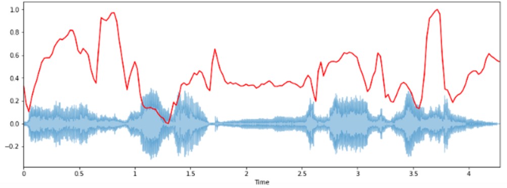
There is a rise in the spectral centroid in the beginning.

2. Spectral Rolloff

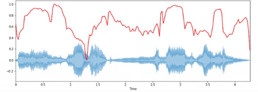
It is a measure of the shape of the signal. It represents the frequency at which high frequencies decline to 0. To obtain it, we have to calculate the fraction of bins in the power spectrum where 85% of its power is at lower frequencies.

librosa.feature.spectral_rolloff computes the roll off frequency for each frame in a signal:

spectral_rolloff = librosa.feature.spectral_rolloff(x+0.01, sr=sr)[0]
plt.figure(figsize=(12, 4))librosa.display.waveplot(x, sr=sr, alpha=0.4)
plt.plot(t, normalize(spectral_rolloff), color='r')

3. Spectral Bandwidth

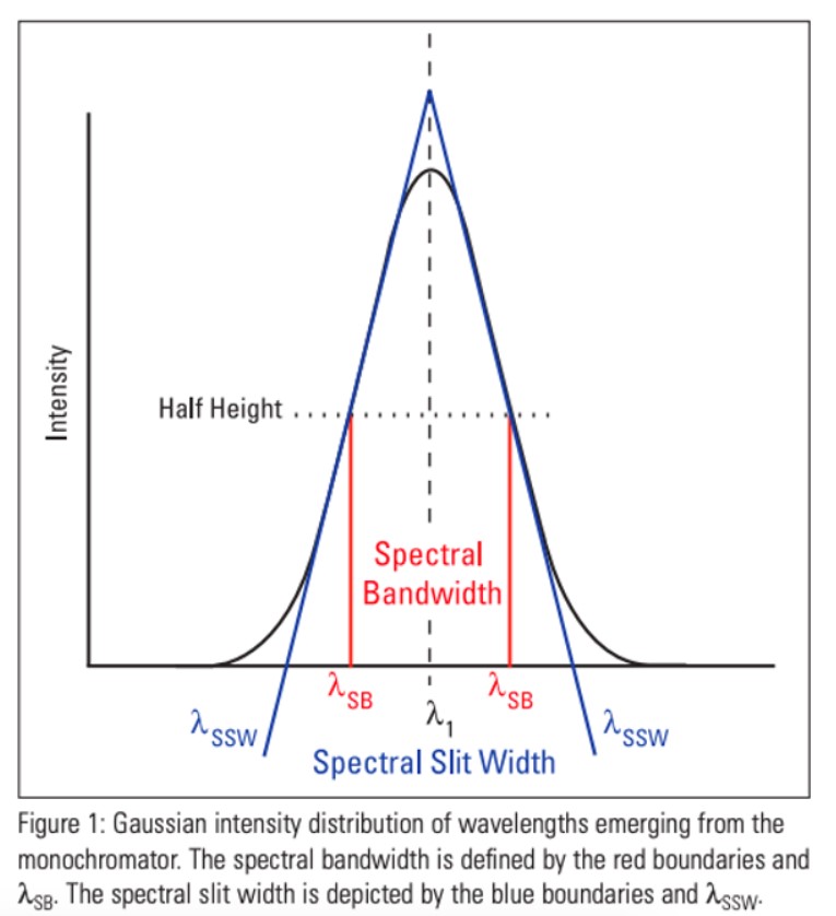
The spectral bandwidth is defined as the width of the band of light at one-half the peak maximum (or full width at half maximum [FWHM]) and is represented by the two vertical red lines and λSB on the wavelength axis.

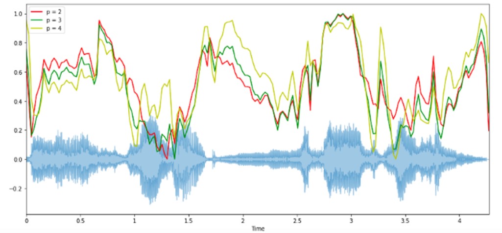
librosa.feature.spectral_bandwidth computes the order-p spectral bandwidth:

spectral_bandwidth_2 = librosa.feature.spectral_bandwidth(x+0.01, sr=sr)[0]
spectral_bandwidth_3 = librosa.feature.spectral_bandwidth(x+0.01, sr=sr, p=3)[0]
spectral_bandwidth_4 = librosa.feature.spectral_bandwidth(x+0.01, sr=sr, p=4)[0]
plt.figure(figsize=(15, 9))librosa.display.waveplot(x, sr=sr, alpha=0.4)
plt.plot(t, normalize(spectral_bandwidth_2), color='r')
plt.plot(t, normalize(spectral_bandwidth_3), color='g')
plt.plot(t, normalize(spectral_bandwidth_4), color='y')
plt.legend(('p = 2', 'p = 3', 'p = 4'))

4. Zero-Crossing Rate

A very simple way for measuring the smoothness of a signal is to calculate the number of zero-crossing within a segment of that signal. A voice signal oscillates slowly — for example, a 100 Hz signal will cross zero 100 per second — whereas an unvoiced fricative can have 3000 zero crossings per second.

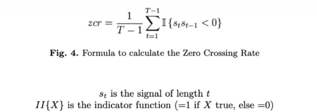
It usually has higher values for highly percussive sounds like those in metal and rock. Now let us visualize it and see how we calculate the zero-crossing rate.

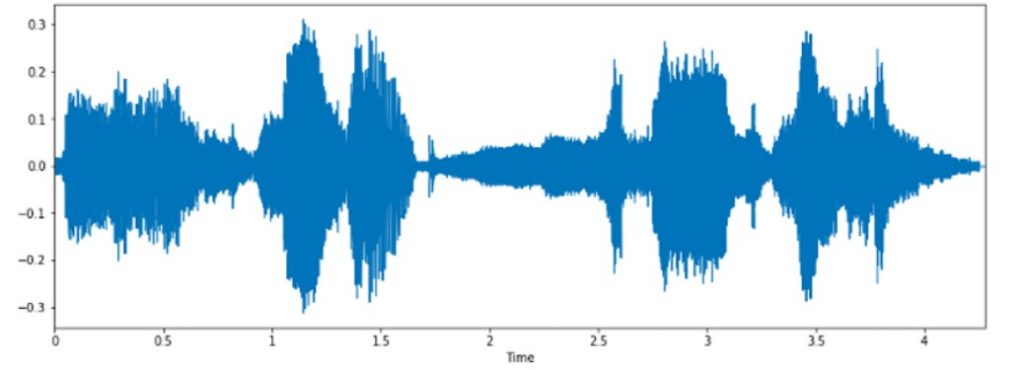
x, sr = librosa.load('/../../gruesome.wav')
#Plot the signal:
plt.figure(figsize=(14, 5))
librosa.display.waveplot(x, sr=sr)
# Zooming in
n0 = 9000
n1 = 9100
plt.figure(figsize=(14, 5))
plt.plot(x[n0:n1])
plt.grid()

Zooming in

n0 = 9000
n1 = 9100
plt.figure(figsize=(14, 5))
plt.plot(x[n0:n1])
plt.grid()

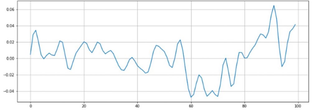
There appear to be 16 zero crossings. Let’s verify it with Librosa.

zero_crossings = librosa.zero_crossings(x[n0:n1], pad=False)
print(sum(zero_crossings))#16

5. Mel-Frequency Cepstral Coefficients(MFCCs)

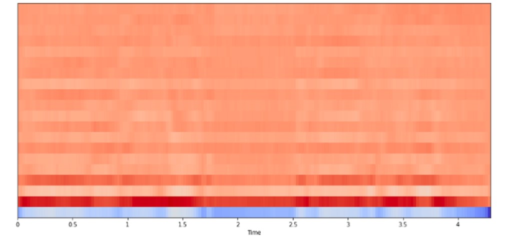
The Mel frequency cepstral coefficients (MFCCs) of a signal are a small set of features (usually about 10–20) that concisely describe the overall shape of a spectral envelope. It models the characteristics of the human voice.

mfccs = librosa.feature.mfcc(x, sr=fs)
print(mfccs.shape)
(20, 97)
#Displaying  the MFCCs:
plt.figure(figsize=(15, 7))
librosa.display.specshow(mfccs, sr=sr, x_axis='time')

6. Chroma feature

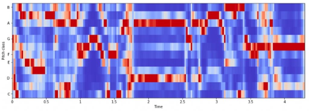
A chroma feature or vector is typically a 12-element feature vector indicating how much energy of each pitch class, {C, C#, D, D#, E, …, B}, is present in the signal. In short, It provides a robust way to describe a similarity measure between music pieces.

librosa.feature.chroma_stft is used for the computation of Chroma features.

chromagram = librosa.feature.chroma_stft(x, sr=sr, hop_length=hop_length)
plt.figure(figsize=(15, 5))
librosa.display.specshow(chromagram, x_axis='time', y_axis='chroma', hop_length=hop_length, cmap='coolwarm')

Now that we understood how we can play around with audio data and extract important features using python. In the following section, we are going to use these features and build an ANN model for music genre classification.

Music genre classification using Artificial Neural Network

Credits

This dataset was used for the well-known paper in genre classification “Musical genre classification of audio signals” by G. Tzanetakis and P. Cook in IEEE Transactions on Audio and Speech Processing 2002.

The dataset consists of 1000 audio tracks each 30 seconds long. It contains 10 genres, each represented by 100 tracks. The tracks are all 22050 Hz monophonic 16-bit audio files in .wav format.

The dataset can be download from marsyas website.

The dataset consists of 10 genres i.e

• Blues
• Classical
• Country
• Disco
• Hip-hop
• Jazz
• Metal
• Pop
• Reggae
• Rock

Each genre contains 100 songs. Total dataset: 1000 songs.

Before moving ahead, I would recommend using Google Colab for doing everything related to Neural networks because it is free and provides GPUs and TPUs as runtime environments.

Roadmap:

First of all, we need to convert the audio files into PNG format images(spectrograms). From these spectrograms, we have to extract meaningful features, i.e. MFCCs, Spectral Centroid, Zero Crossing Rate, Chroma Frequencies, Spectral Roll-off.

Once the features have been extracted, they can be appended into a CSV file so that ANN can be used for classification.

If we wanna work with image data instead of CSV we will use CNN(Scope of part 2).

So let’s begin.

1. Extract and load your data to google drive then mount the drive in Colab.

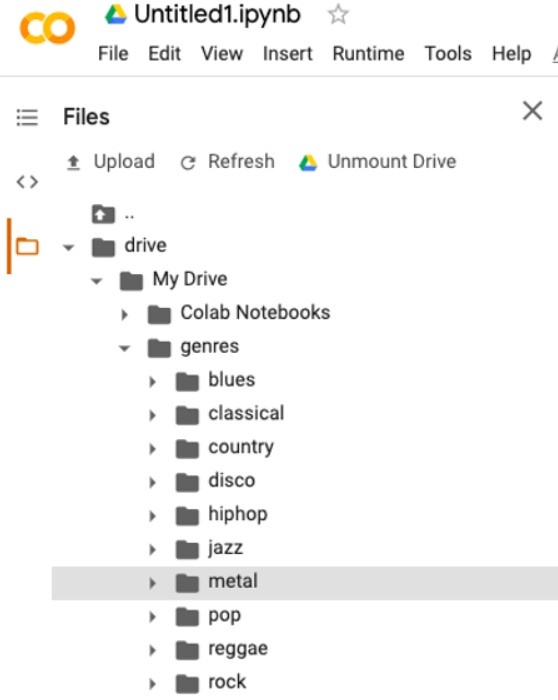
Google Colab directory structure after data is loaded.

2. Import all the required libraries.

import librosa
import pandas as pd
import numpy as np
import matplotlib.pyplot as plt
%matplotlib inline
import os
from PIL import Image
import pathlib
import csvfrom sklearn.model_selection import train_test_split
from sklearn.preprocessing import LabelEncoder, StandardScalerimport keras
from keras import layers
from keras import layers
import keras
from keras.models import Sequentialimport warnings
warnings.filterwarnings('ignore')

3. Now convert the audio data files into PNG format images or basically extracting the Spectrogram for every Audio.

cmap = plt.get_cmap('inferno')
plt.figure(figsize=(8,8))
genres = 'blues classical country disco hiphop jazz metal pop reggae rock'.split()
for g in genres:
    pathlib.Path(f'img_data/{g}').mkdir(parents=True, exist_ok=True)
    for filename in os.listdir(f'./drive/My Drive/genres/{g}'):
        songname = f'./drive/My Drive/genres/{g}/{filename}'
        y, sr = librosa.load(songname, mono=True, duration=5)
        plt.specgram(y, NFFT=2048, Fs=2, Fc=0, noverlap=128, cmap=cmap, sides='default', mode='default', scale='dB');
        plt.axis('off');
        plt.savefig(f'img_data/{g}/{filename[:-3].replace(".", "")}.png')
        plt.clf()

Sample spectrogram of a song having genre as blues.

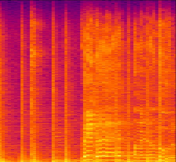
spectrogram of a song having genre as Blues

Now since all the audio files got converted into their respective spectrograms it’s easier to extract features.

4. Creating a header for our CSV file.

header = 'filename chroma_stft rmse spectral_centroid spectral_bandwidth rolloff zero_crossing_rate'
for i in range(1, 21):
    header += f' mfcc{i}'
header += ' label'
header = header.split()

5. Extracting features from Spectrogram: We will extract Mel-frequency cepstral coefficients (MFCC), Spectral Centroid, Zero Crossing Rate, Chroma Frequencies, and Spectral Roll-off.

file = open('dataset.csv', 'w', newline='')
with file:
    writer = csv.writer(file)
    writer.writerow(header)
genres = 'blues classical country disco hiphop jazz metal pop reggae rock'.split()
for g in genres:
    for filename in os.listdir(f'./drive/My Drive/genres/{g}'):
        songname = f'./drive/My Drive/genres/{g}/{filename}'
        y, sr = librosa.load(songname, mono=True, duration=30)
        rmse = librosa.feature.rmse(y=y)
        chroma_stft = librosa.feature.chroma_stft(y=y, sr=sr)
        spec_cent = librosa.feature.spectral_centroid(y=y, sr=sr)
        spec_bw = librosa.feature.spectral_bandwidth(y=y, sr=sr)
        rolloff = librosa.feature.spectral_rolloff(y=y, sr=sr)
        zcr = librosa.feature.zero_crossing_rate(y)
        mfcc = librosa.feature.mfcc(y=y, sr=sr)
        to_append = f'{filename} {np.mean(chroma_stft)} {np.mean(rmse)} {np.mean(spec_cent)} {np.mean(spec_bw)} {np.mean(rolloff)} {np.mean(zcr)}'    
        for e in mfcc:
            to_append += f' {np.mean(e)}'
        to_append += f' {g}'
        file = open('dataset.csv', 'a', newline='')
        with file:
            writer = csv.writer(file)
            writer.writerow(to_append.split())

6. Data preprocessing: It involves loading CSV data, label encoding, feature scaling and data split into training and test set.

data = pd.read_csv('dataset.csv')
data.head()# Dropping unneccesary columns
data = data.drop(['filename'],axis=1)#Encoding the Labels
genre_list = data.iloc[:, -1]
encoder = LabelEncoder()
y = encoder.fit_transform(genre_list)#Scaling the Feature columns
scaler = StandardScaler()
X = scaler.fit_transform(np.array(data.iloc[:, :-1], dtype = float))#Dividing data into training and Testing set
X_train, X_test, y_train, y_test = train_test_split(X, y, test_size=0.2)

7. Building an ANN model.

model = Sequential()
model.add(layers.Dense(256, activation='relu', input_shape=(X_train.shape[1],)))
model.add(layers.Dense(128, activation='relu'))
model.add(layers.Dense(64, activation='relu'))
model.add(layers.Dense(10, activation='softmax'))model.compile(optimizer='adam',
              loss='sparse_categorical_crossentropy',
              metrics=['accuracy'])

8. Fit the model

classifier = model.fit(X_train,
                    y_train,
                    epochs=100,
                    batch_size=128)

After 100 epochs, Accuracy: 0.67

You can also find code on my Github: https://github.com/nageshsinghc4/Audio-Data-Analysis-Using-Deep-Learning

Conclusion

Well, part 1 ends here. In this article, we did a pretty good analysis of audio data. We understood how to extract important features and also implemented Artificial Neural Networks(ANN) to classify the music genre.

In part 2, we are going to do the same using Convolutional Neural Networks directly on the Spectrogram.

I hope you guys have enjoyed reading it. Please share your thoughts/doubts in the comment section.

Thanks for reading.

Note: This article was originally published on theaidream, and kindly contributed to AI Planet (formerly DPhi) to spread the knowledge.