Learning Objectives

• Cost
• Cost Function
• Gradient Descent

Now coming back to our first example. How do you decide what line is good? Here's a bad line:

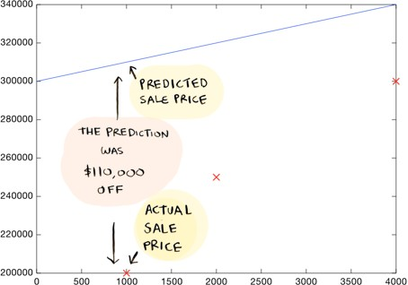
This above-drawn line is way off. For example, according to the line, a 1000 sq foot house should sell for $310,000, whereas we know it actually sold for $200,000.

Here's a better line:

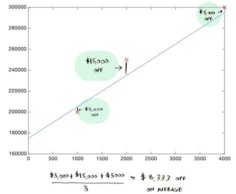
This line is an average of 8,333 dollars off (adding all the distances and dividing by 3).

This $8,333 is called the cost of using this line.

Short-term Objective

What were we doing in the previous two examples? We plotted two straight lines using the equation: y = mx+b.

If we already have the data points (x1, y1), ..., (xn, yn), it means that our values of x and y remain the same throughout all the lines we plot.

So what remains? What exactly are we changing to plot different lines? Yes, m and b.

Our objective is to find the values of m and b that will best fit this data.

These two variables are called hyperparameters. In machine learning, a hyperparameter is a parameter whose value controls the learning process. And we must always try to find optimal parameters while building a machine learning model.

Cost

The cost is how far off the line is from the real data. The best line is the one that is the least off from the real data.

To find out what line is the best line (to find the values of m and b), we need to use a cost function.

In ML, cost functions estimate how badly models are performing.

Put simply, a cost function measures how wrong the model is in terms of its ability to estimate the relationship between X and y.

Cost Function

Now that we built a model, we need to measure its performance, right? and understand if it works well or not. The cost function measures the performance of a Machine Learning model for given data. It quantifies the error between predicted and expected values and presents it as a single real number.

Cost Function can be formed in many different ways depending on the problem. The purpose of this function is to be either:

• Minimized - then returned value is usually called cost, loss, or error. The goal is to find the values of model parameters for which Cost Function returns as small a number as possible.
• Maximized - then the value it yields is named a reward. The goal is to find values of model parameters for which returned number is as large as possible.

What is the predicted and expected value?

• Predicted value: As the name says is the predicted value of your machine learning model.
• Expected value: Is the actual value(or the label present in your data)

Often machine learning models are not 100% accurate or perfect; they tend to deviate from the actual or expected value.

Explaining with an example: If we predict a person's age based on a few input variables or features.

• Our machine learning model predicted the age as 28 years
• However, the actual age of the person is 29 years.
• Here, 28 years is the predicted value, and 29 years is the expected or true value. As data scientists, we try to minimize the error while building models.

Residual is the difference between the true value and the model's predicted value.

Cost Function Types/Evaluation Metrics

There are three primary metrics used to evaluate linear models (to find how well a model is performing):

1. Mean Squared Error
2. Root Mean Squared Error
3. Mean Absolute Error

Mean Squared Error (MSE)

• MSE is simply the average squared difference between the true target value and the value predicted by the regression model.
• As it squares the differences, it penalizes (gives some penalty or weight for deviating from the objective) even a small error which leads to over-estimation of how bad the model is.

Root Mean Squared Error (RMSE)

• It is just the square root of the mean square error.
• It is preferred in some cases because the errors are first squared before averaging, which poses a high penalty on large errors. This implies that RMSE is useful when large errors are undesired.

Mean Absolute Error(MAE)

• MAE is the absolute difference between the target value and the value predicted by the model.
• MAE does not penalize the errors as effectively as MSE, making it unsuitable for use-cases where you want to pay more attention to the outliers.

R-Squared (Coefficient of Determination)

• R-squared is a goodness-of-fit measure for linear regression models.
• It represents the coefficient of how well the values fit compared to the original values. The values from 0 to 1 are interpreted as percentages.
• The higher the value is, the better the model is.
  
  Where = predicted value of y,
  = mean value of y
• Going by the name, you might think R2 cannot be negative. However, it can. A Negative R2 means you are doing worse than the mean value.

Which metrics to use when?

This is an important question, and we get used to learning these measures over time. Sharing some resources with you all so that it helps you understand what metrics to be used in the context of solving a regression problem.

• https://medium.com/usf-msds/choosing-the-right-metric-for-machine-learning-models-part-1-a99d7d7414e4
  (you may ignore the "Bonus" section in the article for the time being)

Note: Gradient Descent is a slightly advanced topic. Feel free to skip it if you don't want to go into maths.

Gradient Descent

The gradient is another word for "slope". The higher the gradient of a graph at a point, the steeper the line is at that point. A negative gradient means that the line slopes downwards.

Finding the gradient of a straight-line graph

It is often useful or necessary to find out what the gradient of a graph is. For a straight-line graph, pick two points on the graph. The gradient of the line = (change in y-coordinate)/(change in x-coordinate) .

In this graph, the gradient = (change in y- coordinate)/(change in x-coordinate)
= (8- 6)/(10-6)
= 2/4 = 1/2

We can, of course, use this to find the equation of the line. Since the line crosses the y-axis when y = 3, the equation of this graph is y = ½x + 3.

Finding the gradient of a curve

To find the gradient of a curve, you must draw an accurate sketch of the curve. At the point where you need to know the gradient, draw a tangent to the curve. A tangent is a straight line that only touches the curve at one point. You then find the gradient of this tangent.

example

Find the gradient of the curve y = x² at the point (3, 9).

Gradient of tangent = (change in y)/(change in x)
= (9 - 5)/ (3 - 2.3)
= 5.71

The cost function will tell you how good those values are (i.e., it will tell you how far off your predictions were from the actual data). But what do we do based on that information? How do we find the values of m and b that will draw the best line? By using gradient descent.

In a nutshell, to update m and b values to reduce Cost function (minimizing RMSE value) and achieve the best fit line, the model uses Gradient Descent. The idea is to start with random m and b values and then iteratively update the values, reaching minimum cost.

Let's start with a simpler version of gradient descent and then move on to the real version.

Suppose we decide to leave b at zero. So we experiment with what value m should be, always keeping b at 0. Now you can try various values for m, and you will end up with different costs. You can plot all of these costs on a graph:

Here are the corresponding lines (remember, b is zero in these lines):

We can see that the line on the left seems to fit the data better than the line on the right, so it makes sense that the cost of that line is lower. And from this graph, it looks like m = 75 gives us the lowest cost overall.

Since it is the lowest point in this graph, with all the costs graphed out like this, we need to find the lowest point on the graph, which will give us the optimal value of m!

Gradient descent helps us find the lowest point on this graph. You start with a value for m and update it iteratively till you arrive at the best value. So you can begin at m = 0. Then you have to ask, should I go left or right?

Well, we want to go down, so let's go right a small step:

This is the new value for m. Again we ask, should we go left or right? At each step, you need to head down till you get to a point where you're as low as you can go:

This is gradient descent: going down until you hit the bottom.

How do you figure out which way is down? The answer will be obvious to calculus experts but not so obvious for the rest of us: you take the derivative at that point.

But the important bit to know is that if you take the current value of m and add the derivative at that point, you will go down. You do that a bunch of times (say 1000 times), and you will hit bottom!

The video below explains the process of gradient descent. You only need to watch till 16:07 to gain some understanding and not go into the python implementation explained later on.

Also, as the instructor said, there's no need to dive into the mathematics or worry about not understanding some math right now.

Recap

• Linear regression is used to predict a value (like the sale price of a house).
• Given a data set, first try to fit a line.
• The cost function tells you how good your line is.
• You can use gradient descent to find the best line.

Slide Download Link

You can download the slides for this topic from here.