Learning Objectives

• Statistics
• Data Types in Statistics (Important)
• Measures of Central Tendencies
• Measures of Dispersion
• Transformations
• Distribution

Statistics

What is Statistics?

A branch of mathematics that takes and transform the data into some useful information which in turn is used to make some decisions.

Statistics is concerned with:

• Processing and analyzing data
• Collecting, presenting and transforming data to assist decision maker

Data

What is Data?

Data are facts and statistics collected together for reference or analysis.

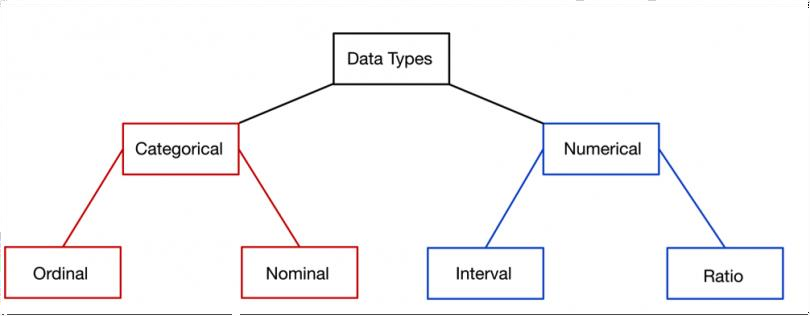
Categorical

• Nominal: Doesn’t have an order. For example: Gender of a person (male or female)

• Ordinal: Has some order in place. For example: Grades of students (first division, second division and third division)

Numerical

• Discrete: Discrete Data can only take certain values. They are distinct and separate.
  Example: the number of students in a class. We can't have half a Student!

• Continuous: Continuous Data can take any value (within a range).
  A person's height: could be any value (within the range of human heights), not just certain fixed heights.

Note: we will get used to these terms soon, no need worry too much about it. Read this article for additional information:
https://builtin.com/data-science/data-types-statistics

Measures of Central Tendency

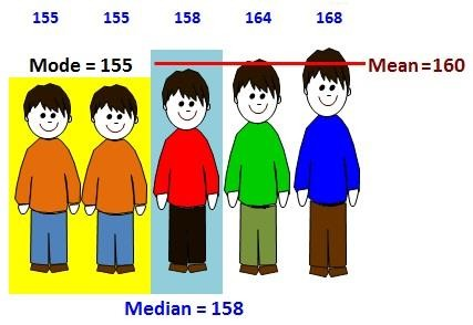
• Mean: The mean is the average of a data set. For example, take a list of numbers: 10, 20, 40, 10, 70
  Mean = (10 + 20 + 40 + 10 + 70) / 5 = 30
• Median: The median is the middle of the set of numbers. To find the median, first we sort the list of numbers:
  10, 10, 20, 40, 70
  The exact middle number i.e. 20 is the median.
• Mode: The mode is the most common number in a data set.
  In above list of numbers, 10 has occurred 2 times while other three numbers are occurred one time each.
  So, the mode is 10 here.

Applications of Central Tendencies

MEAN: When you watch a baseball game and you see the player's batting average, that number represents the total number of hits divided by the number of times at bat. In other words, that number is the mean. In school, the final grade you get in a course is usually a mean. This mean represents the total number of points you scored in the class divided by the number of possible points. This is the classic type of average – when your overall performance on many items is evaluated with a single number.

MEDIAN: Although the mean is the most common type of average, the median can also be used to express the average of a group. You may hear about the median salary for a country or city. When the average income for a country is discussed, the median is most often used because it represents the middle of a group. Mean allows very high or very low numbers to sway the outcome but median is an excellent measure of the center of a group of data.

MODE: Imagine that you live in a small town where most of the people are employed by a factory and earn minimum wage. One of the factory owners lives in the town and his salary is in the millions of dollars. If you use a measure like the average to try to compare salaries in the town as a whole, the owner's income would severely throw off the numbers. This is where the measure of mode can be useful in the real world. It tells you what most of the pieces of data are doing within a set of information.

Measures of Dispersion

• Range: It is the difference between highest value and the lowest value in the data set.
  For a given list of numbers: 10, 20, 40, 10, 70 the range is 70 - 10 = 60.
• Variance: The average of the squared differences from the mean. Steps to calculate variance:
  • Calculate mean (mean is nothing but average)
  • Find difference of each data from mean
  • Square all the differences
  • Take the average of the squares.
• Standard Deviation: It shows you how much your data is spread out around the mean. Its symbol is ???? (the greek letter sigma). It is the square root of the variance.

Consider the list of numbers: 10, 20, 40, 10, 70.

• Mean of the number is 30.
• Difference of each data from the mean: -20, -10, 10, -20, 40.
• Square of all the differences: 400, 100, 100, 400, 1600
• Take the average of the squares:
  (400 + 100 + 100 + 400 + 1600) / 5 = 2600 / 5 = 520

Standardization/Normalization

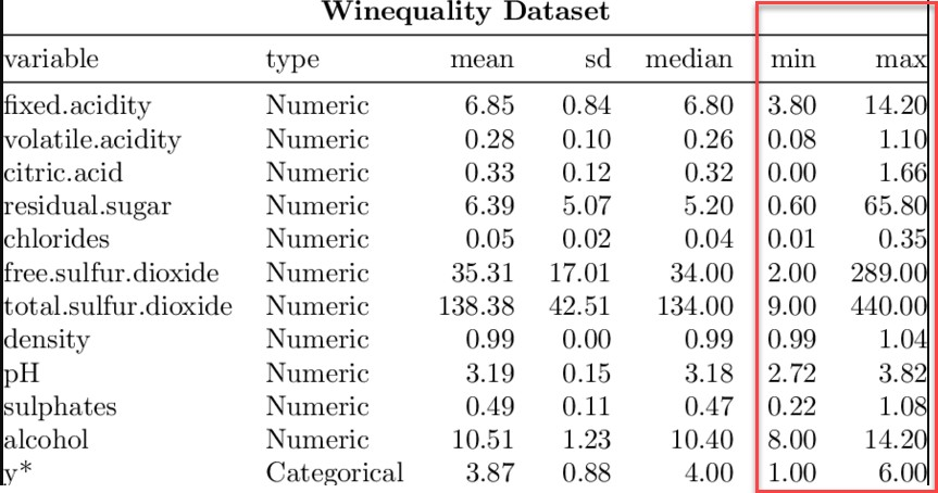
Often variables in a real dataset come with a wide range of data values.

For example let’s look at the wine dataset given in next slide, the fixed.acidity variable has values ranging from 3.8 to 14.2. Similarly, if we look at volatile.acidity, it has values ranging from 0.08 to 1.10. Basically, they are not on a common scale.

Now how does standardization/normalization help? Performing standardization/normalization would bring all the variables in a dataset to a common scale to further help implement various machine learning models (where standardization/normalization is a pre-requisite to apply such models). Again, don’t take this for granted, there are some smart algorithms which doesn’t need this and we will explore them soon!

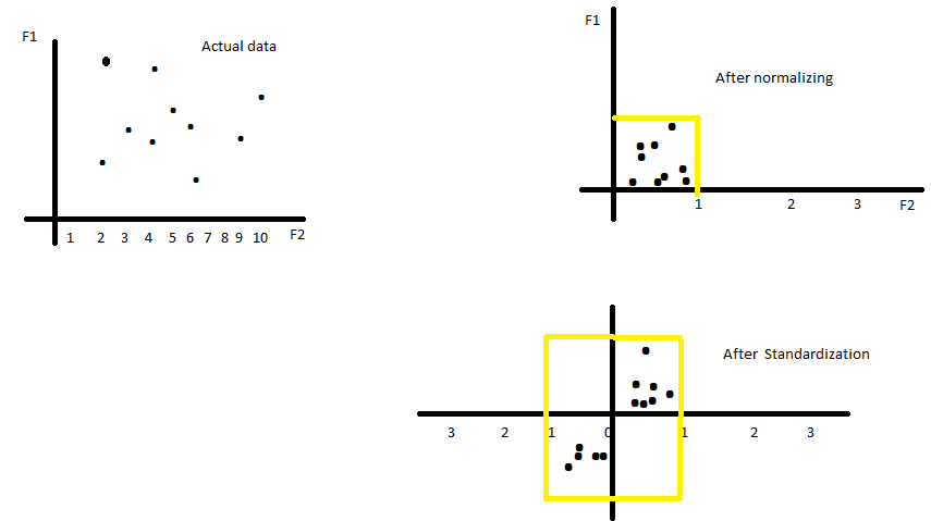
Look at the above graphs. The actual data is scattered across a wide range.

Normalisation helps in bringing the whole data within a particular range.

Standardisation distributes the data in a manner such that it now has a mean of 0 and standard deviation of 1.

Transformation

Some machine learning algorithms are quite sensitive to the scale of the numeric values provided.

Consequently, in order for the algorithm to converge faster or to provide a more exact solution, rescaling the distribution is necessary. Rescaling mutates the range of the values of the features and can affect variance, too. You can perform features rescaling in two ways:

1. Using statistical standardization (z-score normalization) Standardization typically means rescaling data to have a mean of 0 and a standard deviation of 1 (unit variance).
2. Using the min-max transformation (or normalization) Normalization typically means rescaling the values into a range of [0,1].

Distribution

• Probability - by going with the literal meaning it is the extent to which something is likely to happen or probable. The same concept applies to statistics when we talk about probability distributions.
• A probability distribution is a function that describes the likelihood of obtaining the possible values (probability) of a variable.
• Suppose a teacher notes down the heights of all students in her class.
• Now, she can draw a probability distribution when she needs to know which outcomes (heights) are most likely, the spread of potential values (range of heights), and the likelihood of different results (probability of each height).

• Let’s take the heights dataset consisting of student IDs and heights:
  https://bit.ly/Heights_Data

• The most convenient way to take a quick look at a distribution in seaborn is the distplot() function. On plotting a distplot on this dataset, we’ll observe a bell shaped curved like this:

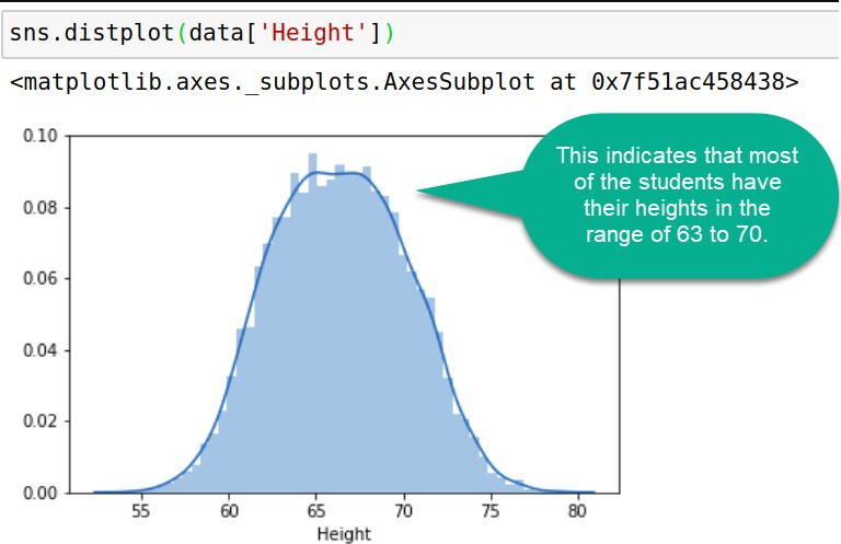
• Probability distributions are usually (but not solely) represented in charts whose abscissa axis ( x axis) represents the possible values of the variable and whose ordinal axis ( y axis) represents the probability of occurrence (probability density).

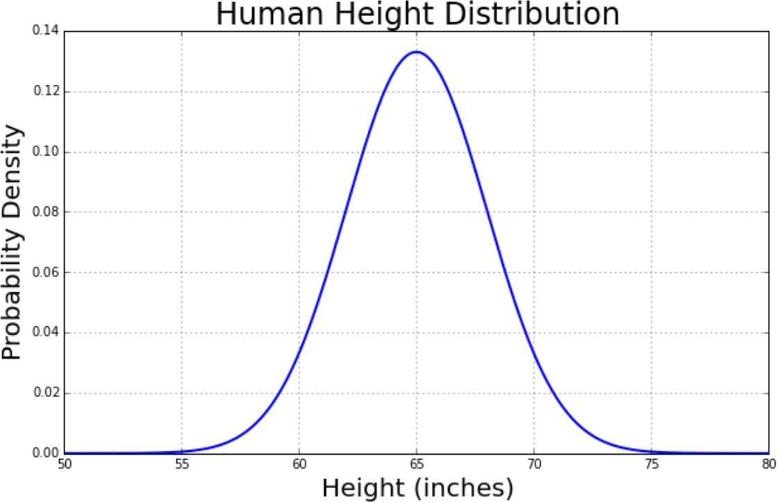
• Most statistical models rely on a normal distribution, a distribution that is symmetric and has a characteristic bell shape.

Normal/ Gaussian Distribution

• Also called bell shaped curve.
• It is a distribution of data that occurs naturally in many situations.
• It is a probability distribution that is symmetric about the mean, showing that data near the mean are more frequent in occurrence than data far from the mean.

Skewness

• Real life data rarely, if ever, follow a perfect normal distribution.
• The skewness measures the symmetry of a distribution or how different a given distribution is from a normal distribution.
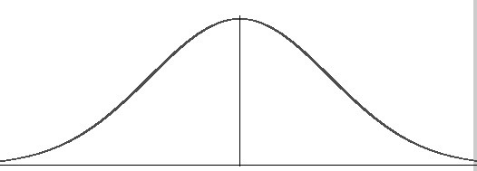
• The normal distribution is symmetric and has a skewness of zero.
• There are two types of Skewness: Positive and Negative

• Positive/Right Skewness means when the tail on the right side of the distribution is longer or fatter. The mean and median will be greater than the mode.
• Negative/Left Skewness is when the tail of the left side of the distribution is longer or fatter than the tail on the right side. The mean and median will be less than the mode.
• For further reading refer: https://www.statisticshowto.com/probability-and-statistics/skewed-distribution/

Understanding skewness with an example

• Let us take a very common example of house prices. Suppose we have house values ranging from 1,000,000 with the average being $500,000.
• If the peak of the distribution was left of the average value, portraying a positive skewness in the distribution. It would mean that many houses were being sold for less than the average value, i.e. $500k. This could be for many reasons, but we are not going to interpret those reasons here.
• If the peak of the distributed data was right of the average value, that would mean a negative skew. This would mean that the houses were being sold for more than the average value.

Slide Download Link

You can download the slides for this topic from here.