Before we jump into RNN math, it is important to look at the previous layer that is involved before the RNN layer.
Let's take an example:
- "AI Planet Bootcamps are free and available to all."
Step 1: Tokenization
During this step, we first, make each unique word as a single token:
['AI','Planet','Bootcamps','are','free','and','available','to','all']
Once this is done we assign each token with the index i.e., each word is now a Vocabulary. The vocab size is very important for embedding layer
1 2 3 4 5 6 7 8 9 10 11{ "AI": 1 "Planet": 2 "Bootcamps": 3 "are": 4 "free": 5 "and": 6 "available": 7 "to": 8 "all": 9 }
So, our sentence becomes: [1, 2, 3, 4, 5, 6, 7, 8, 9].
Step 2: Embedding layer
In NLP, we usually convert words into dense vectors that capture their semantic meaning. This is like giving each word a unique "signature".
Assuming an embedding size of 3 (just for simplicity), the word "AI" might be represented as
1
[0.1, 0.2, 0.3] In the real-time example, the Embedding size varies from 128 to 1024.
Now the entire 'AI Planet bootcamps are free and available to all' sentence becomes:
1 2 3 4 5 6[[0.1, 0.2, 0.3], [0.4, 0.5, 0.6], [0.7, 0.8, 0.9], ... [0.7, 0.8, 0.9], [0.4, 0.5, 0.6]]
Step 3: RNN Layer - Math Simplified
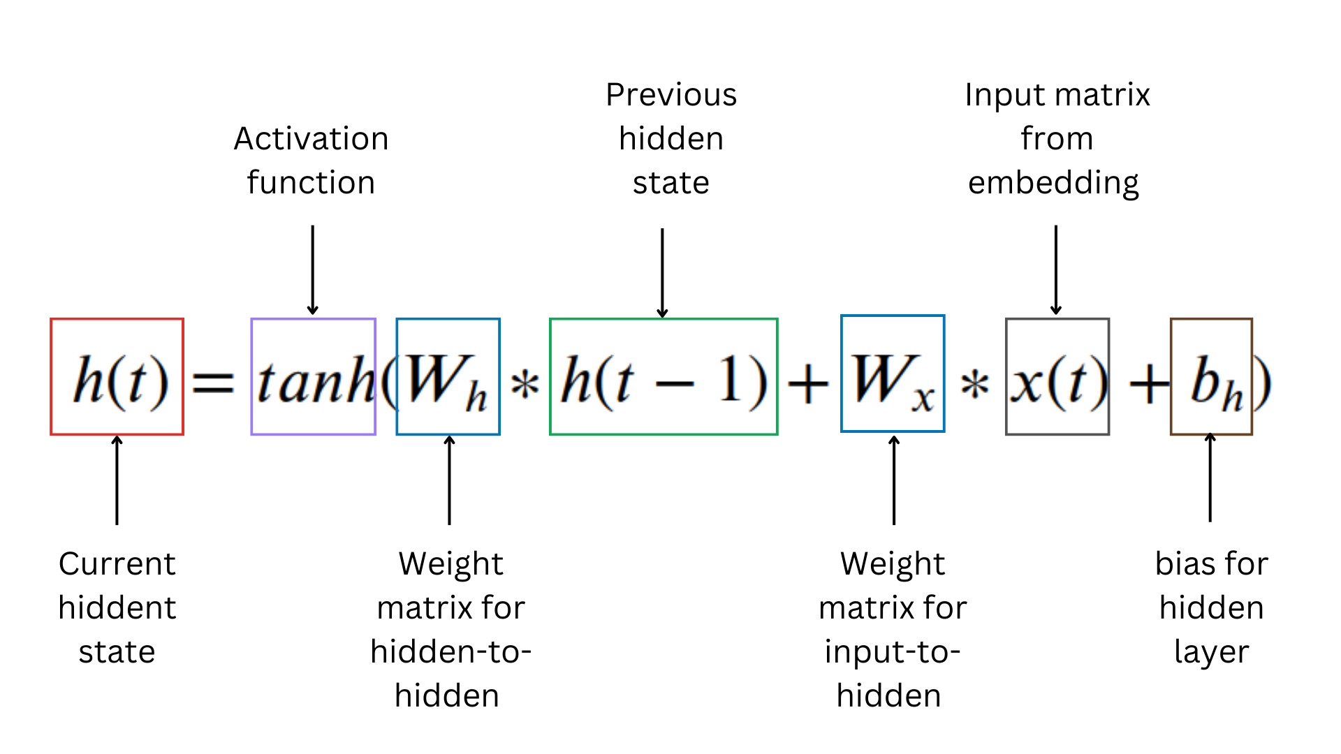
Underestanding the Notations involved in RNN:
- t: denotes the time step
- h(t): denotes the hidden state to current time step
- h(t-1): denotes the previous hidden state at time step t-1
- x(t): denotes the input at time step t. This is the input that is received from embedding layer. In the below example observe carefully, the shape matches with that of embedding
- tanh: Is the activation function that is used to calculate the next hiddent state value i.e., h(t) in dependent to h(t-1)
The RNN processes the sequences step by step, maintaining an internal state that captures information from previous time steps.
We need to define the hidden state size [hyperparameter]. Assume our RNN has a hidden state size of 2.
Let's simplify the RNN math for one time step.
Given an input at time step t, denoted as x(t), and the previous hidden state at time step t-1, denoted as h(t-1), the calculations in the RNN are as follows:
1. Calculate the new hidden state and output:
Note: When we calculate h(1), the initial hidden state value h(0) is filled with zeroes.
2. Initial hidden state (h(0)):
1[0, 0]
Sample Python code snippet
1ht = np.zeros((self.hidden_size,1))
3. Initialize weight matrix randomly
a)
1 2[[0.1, 0.2], [0.3, 0.4]]
b)
1 2[[0.5, 0.6, 0.7], [0.8, 0.9, 1.0]]
c)
1 2[[0.2, 0.3], [0.4, 0.5]]
Note: A kind reminder, the weights are usually initialized randomly. Also notice the size of the weight matrix is 2x3 that is corresponding to hidden_size x embedding_size
Sample Python Code snippet
1 2 3Wx = np.random.randn(self.hidden_size, self.input_size.shape[2]) Wh = np.random.randn(self.hidden_size, self.hidden_size) Wy = np.random.randn(self.output_size.shape[1],self.hidden_size)
Bias
- Bias for hidden state (b_h):
1[0.1, 0.2]
- Bias for output (b_y):
1[0.3, 0.4]
Step 3. Calculate the new hidden state h(1) and the output y(1) at the first time step
We have total 9 vocabulary in the Embeddings, let's just take the first word (x(1)):
1[0.1, 0.2, 0.3]
Now let's Calculate the weighted sum of the previous hidden state (h(0)) and the input (x(1)) along with the bias for the hidden state: (b(h)):
1 2 3 4 5 6 7 8 9weighted_sum = W_h * h(t-1) + W_x * x(t) + b_h weighted_sum = [[0.1, 0.2], [0.3, 0.4]] * [0, 0] + [[0.5, 0.6, 0.7], [0.8, 0.9, 1.0]] * [0.1, 0.2, 0.3] + [0.1, 0.2] = [0.0, 0.0] + [0.38, 0.56] + [0.1, 0.2] = [0.48, 0.76]
Let's apply tanh function and find out h(1)
1 2h(1) = tanh([0.21, 0.46]) ≈ [0.44624361, 0.64107696]
Let's apply sigmoid function and find out y(1)
- y(t) = sigmoid(W_y⋅h(t)+b_y)
Calculate:
1 2 3 4y(1) = sigmoid([[0.2, 0.3], [0.4, 0.5]] * [0.206, 0.440] + [0.3, 0.4]) = sigmoid([0.216, 0.355] + [0.3, 0.4]) = sigmoid([0.516, 0.755]) ≈ [0.61614087, 0.66871967]
Verification via code
1 2 3import numpy as np W_hXh_t_1 = np.dot(np.array([[0.1, 0.2], [0.3, 0.4]]),np.array([0, 0]))
1 2W_xXx_t = np.dot(np.array([[0.5, 0.6, 0.7], [0.8, 0.9, 1.0]]),np.array([0.1, 0.2, 0.3]))
1b_h = np.array([0.1, 0.2])
1 2weighted_sum = W_hXh_t_1 + W_xXx_t + b_h weighted_sum
1array([0.48, 0.76])
1 2h_1 = np.tanh(weighted_sum) h_1
1array([0.44624361, 0.64107696])
1 2def sigmoid(x): return 1 / (1 + np.exp(-x))
1 2 3 4 5 6 7 8y_1 = sigmoid( np.dot( np.array([[0.2, 0.3], [0.4, 0.5]]), np.array([0.206, 0.440]) ) + np.array([0.3, 0.4]) ) y_1
1array([0.61614087, 0.66871967])
Step 5. Loss Function:
The loss function measures the difference between the predicted output and the actual target output. In the context of sequence tasks like language modeling, sentiment analysis, or sequence-to-sequence tasks, a common choice for the loss function is the categorical cross-entropy loss.
L(t) = - sum(y_actual(t) * log(y(t)))
Here let's say our use case is sentiment anaylsis, considering our example "AI Planet Bootcamps are free and available to all." is a positive sentiment
thus:
y_actual = 1
Step 6. Backwardpropogation through time (BPTT):
-
First we calculate forward pass as above
-
Then we calculate the loss for each time step using the predicted outputs (y(t)) and the true target outputs(y(actual)).
-
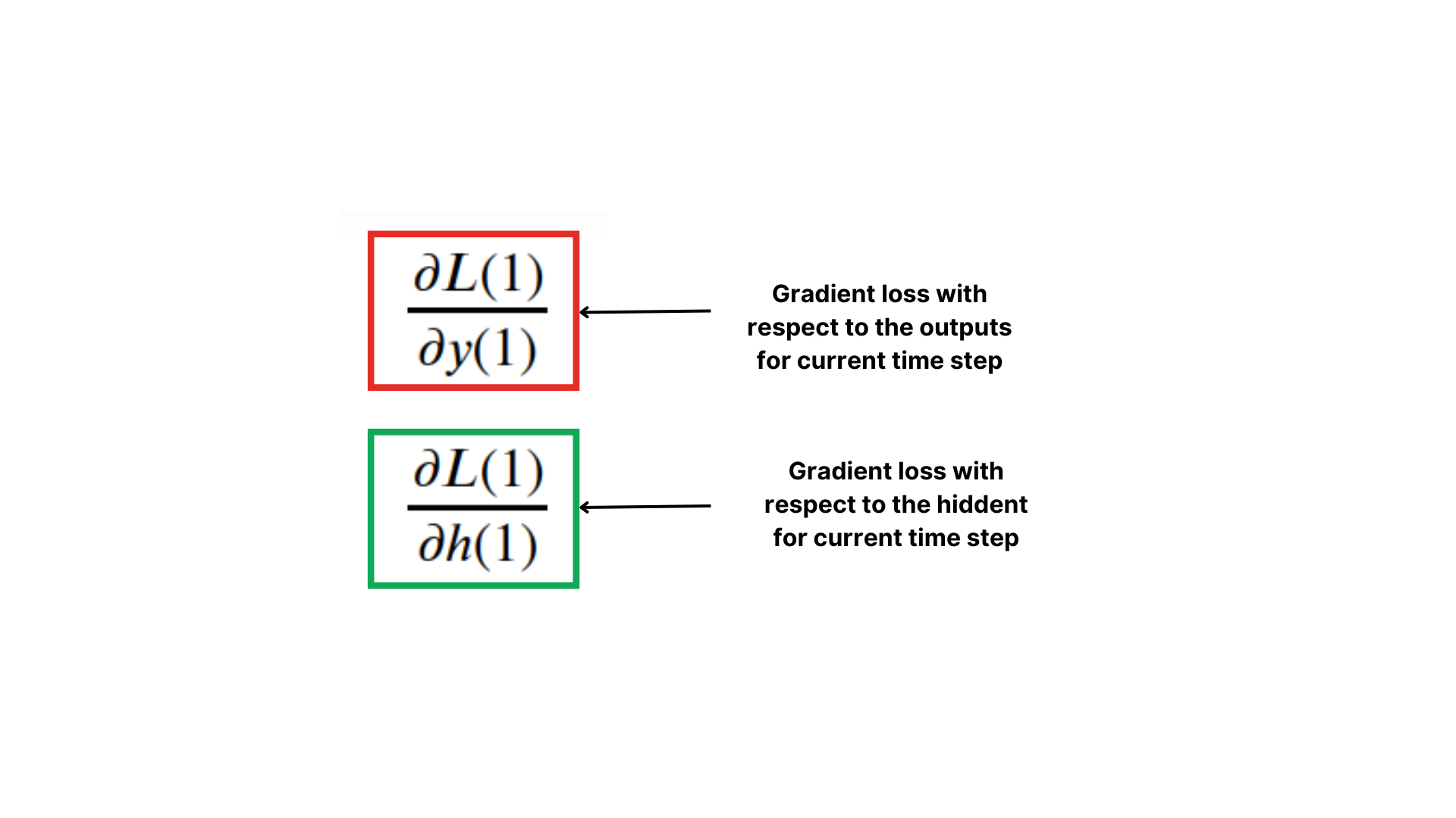
Begin the backpropagation process by computing the gradient (partial derivations) of the loss with respect to the outputs and hidden states at the last time step (T).
-
Iterate backward through time steps from T down to 1. For each time step t, calculate the gradients of the loss with respect to the hidden state and input at time step t, and update the gradients with respect to the parameters (W_x, W_h, W_y, biases, etc.).
-
Use learning rate to add the step size to update the weights (W_x, W_h, W_y).
-
Continue iterating over mini-batches of sequences and performing forward and backward passes until convergence i.e., end of time step or a specified number of epochs.
Sample Python code snippet
1 2 3 4 5 6 7 8 9 10 11 12 13 14 15 16 17 18 19dWy = np.dot(dyt,self.hidden_states[-1].T) dht = np.dot(dyt, self.Wy).T dWx = np.zeros(self.Wx.shape) dWh = np.zeros(self.Wh.shape) for step in reversed(range(n)): temp = (1-self.hidden_states[step+1]**2) * dht dWx += np.dot(temp, self.inputs[step].T) dWh += np.dot(temp, self.hidden_states[step].T) dht = np.dot(self.Wh, temp) #gradient clipping: this is used to tackle Exploding Gradient problem dWy = np.clip(dWy, -1, 1) dWx = np.clip(dWx, -1, 1) dWh = np.clip(dWh, -1, 1) #weights updation using learning rate(step size) self.Wy -= self.lr * dWy self.Wx -= self.lr * dWx self.Wh -= self.lr * dWh