Learning Objectives

• Story time of ANN & Non-Linear Boundary
• Neural Network Architecture
• Forward Propagation
• Gradient Descent - Refresher
• Backpropagation

The Story of a Neural Network, also known as Artificial Neural Network - ANN.

ANN

ANN is a unique computer who doesn't want to be programmed like others. She wants to learn independently, even if it takes longer and involves a lot of trial and error. Was she able to succeed? Watch the video to find out.

Classification

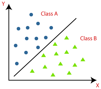
• Classification divides the given data points into two or more classes.
• For example, in the given image, we classify the data into classes A and B.
• The data in the image are classified with a straight line (i.e., linear boundary)

Non-linear Boundary

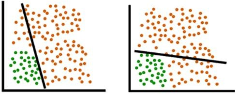
Both the models above cannot classify our data into two classes because, in both cases, the red points (significant in number) are present on both sides of the line.

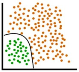
We thus need something better than a straight line to divide our data into two separate classes.

Realistic data is much more complex and not always classified by a straight line. For this purpose, we need a non-linear boundary to separate our data. The perceptron model works on the most basic form of a neural network, but we use Deep Neural Network or Multi-Layer Perceptrons for realistic data classification.

Neural Network Architecture

• Neural Networks are complex structures made of artificial neurons that can take in multiple inputs to produce a single output.
• This is the primary job of a Neural Network
• Simple terms, to transform input into a meaningful output
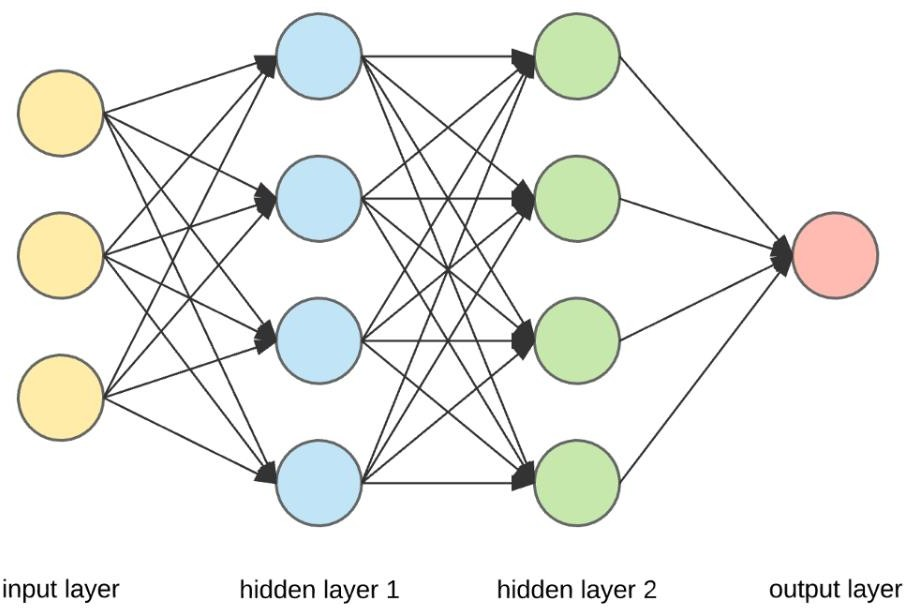
• NN consists of an input and output layer with one or more hidden layers.

Neural Network Components

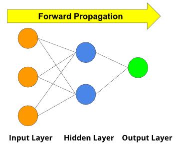
• Outermost yellow layer is the input layer. A neuron is the basic unit of a neural network. In this case, the input layer has three neurons. The inputs are simply the measure of our features. For example, in the Boston house price data in the Linear Regression with tf.keras notebook, there were 13 input features, so the input layer will have 13 neurons.

• The blue and green layers are two hidden layers that are not directly observable while building the neural network. We initially assign the number of neurons in these hidden layers, and we can find the optimal number of neurons in the hidden layer through hyperparameter tuning.

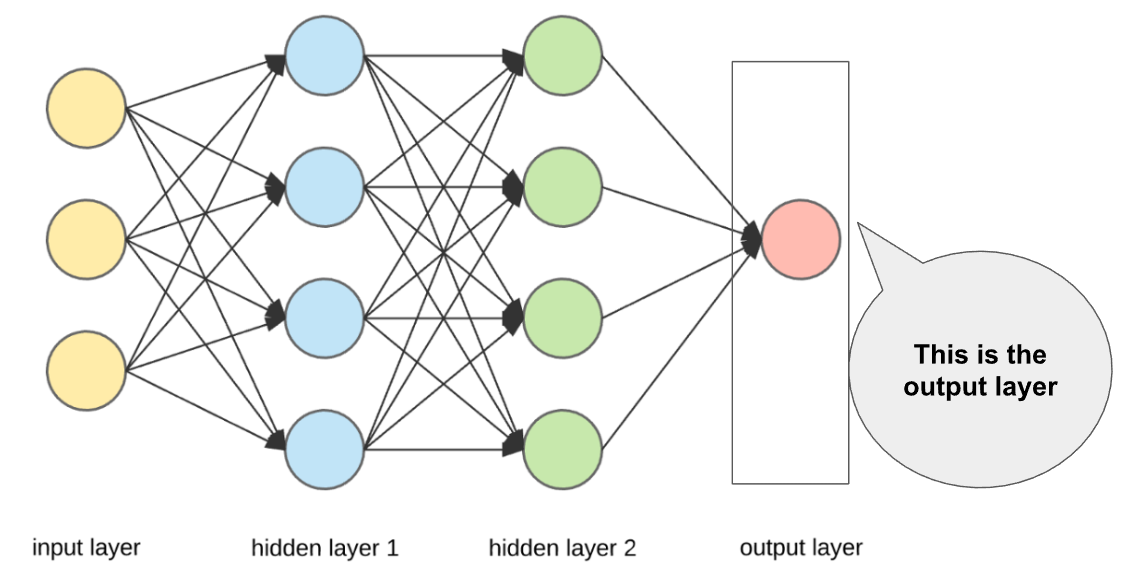
Image source: UpGrad

• The red layer is the output layer. This is the last layer of a neural network that produces the required output. For example, 'MEDV' (Median value of owner-occupied homes in 1000's USD) was the output layer in boston house price dataset.

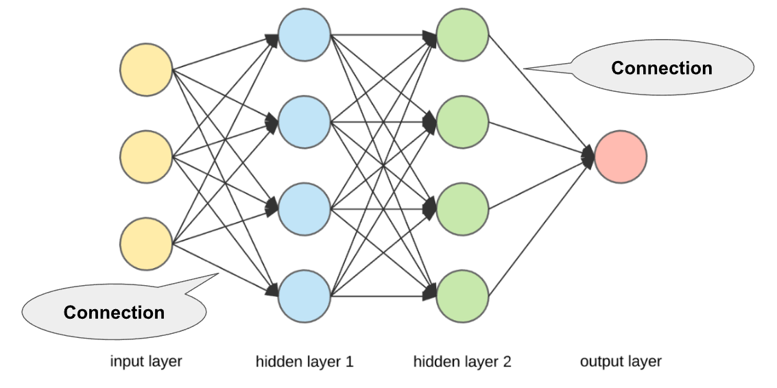
• Weights: There is some weight assigned for each connection. Weights represent scalar (constant) multiplication. Initially, these are assigned randomly; then, these weights are updated as per their importance in predicting the output. The updation of weight is done through Backpropagation (you will know this soon).

• Now, we know each neuron in the input layer has a value given in the dataset. Some random weights are assigned for each connection. We multiply the value of each neuron with the weight for the next connecting neuron and add them all together, producing the value of the next connecting neuron in the next layer. Don't worry if you don't understand here. An example of this calculation is shown in the next section.

Calculating Value of a Neuron

A simple example of how the values of each neuron are calculated using weights and input values.

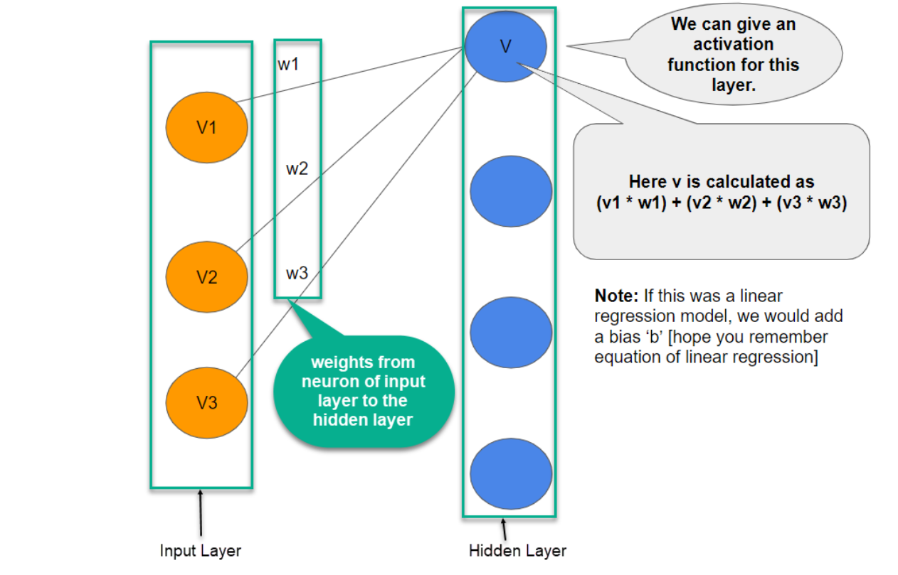
• In the above image: w1 is the weight from the input layer's first neuron to the hidden layer's first neuron. The same goes with w2 and w3.
• The value of each other neuron in each hidden layer is calculated the same way we calculated the value of the first neuron of the first hidden layer in the previous image.
• Similarly, the value of the output layer is calculated.

Let's understand what we learned using a simple task.

Task - Making tea

Now imagine you are a Tea Master. The ingredients used to make tea (water, tea leaves, milk, sugar, and spices) are the "neurons" since they make up the starting points of the process. The amount of each ingredient represents the "weight." Once you put the tea leaves in the water and add the sugar, spices, and milk in the pan, all the ingredients will mix and transform into another state. This transformation process represents the "activation function."

Hidden Layers and output Layer

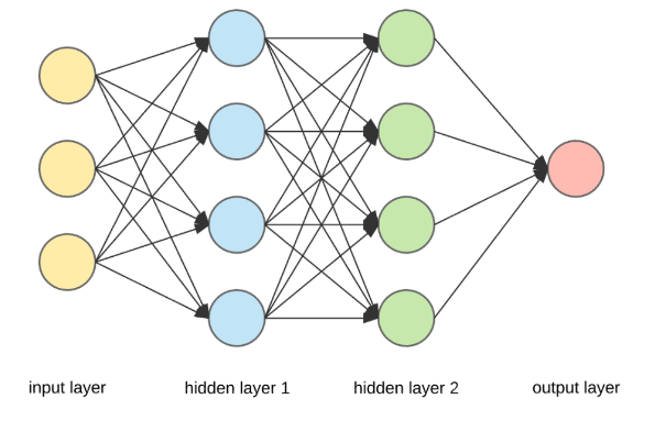
• The layers hidden between the input and output layer are known as the hidden layers. It is called the hidden layer since it is always hidden from the external world. The main computation of a Neural Network takes place in the hidden layers. So, the hidden layer takes all the inputs from the input layer and performs the necessary calculation to generate a result. This result is then forwarded to the output layer so the user can view the computation result.
• In our tea-making example, when we mix all the ingredients, the formulation changes its state and color on heating. The ingredients represent the hidden layers. Here heating represents the activation process that finally delivers the result – tea.

Summary of Tea Example

• Input layers: water, tea leaves, sugar, milk, and spices
• Hidden layers: all the above ingredients mixed with certain weights
• Activation function: The heating process
• Output layer: Tea

Another intuitive Explanation of Neural Networks

Explanation of Neural Networks (Optional)

If you like understanding things through Mathematics, this is for you! ????

Working of a Neural Network

In the upcoming sections, we will be discussing the working of Neural Networks, which includes three main steps:

1. Forward Propagation
2. Gradient Descent
3. Backward Propagation

What are they? These are the three important pillars of the neural network, and we will learn more about their prominence now.

Why Forward Propagation in NN?

• We need to feed input data to generate output or desired results. Forward propagation helps us do that in Neural Networks. The data in NN should be fed in the forward direction only.

Why Gradient Descent?

• Think of Gradient Descent as a technique to minimize the loss/cost function. It helps in making the model perform better.

Why Backward Propagation in NN?

• When you generate some output through forward propagation, some errors are generated. To reduce these errors, we traverse back from the output layer to the input layer and update the initially assigned weights.

Forward Propagation

What is Forward Propagation in NN?

• Well, if you break down the words, forward implies moving ahead, and propagation is a term for saying spreading of anything.
• Forward propagation means moving in only one direction in a neural network, from input to output.

The video below takes a Bank Transaction Dataset Example. The dataset has two features; the number of children and accounts, and the objective is to predict how many transactions a user will make at the bank.

The video covers the following aspects:

• How neural network model uses data to make predictions
• How the information is transferred from the input layer to the output layer (through weights and hidden layers)
• The calculation of the value of each neuron in hidden layers using weights and the input values
• And finally, calculating the output

Note: In the video, the inputs (2,3) and weights (1, -1, etc.) are randomly assigned for an explanation. NO need to bother to know how they started appearing all of a sudden!

Gradient Descent

Gradient Descent (GD) is an optimization technique in the machine learning process that helps us minimize the cost function by learning the model weights to fit the training data well.

Gradient = rate of inclination or declination of a slope (how steep a slope is and in which direction it is going) of a function at some point.

Descent = an act of moving downwards.

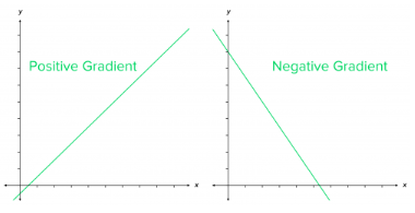
A simple way to memorize:

• line going up as we move right → positive slope/gradient
• line going down as we move right → negative slope/gradient

Gradient Descent - A technique to minimize cost

• At the start, the parameter values of the hypothesis are randomly initialized (can be 0)
• Then, Gradient Descent iteratively (one step at a time) adjusts the parameters and gradually finds the best values for them by minimizing the cost
• In this case, we'll use it to find the parameters m and c of the linear regression model
• m = slope of a line that we just learned about
  c = bias/intercept: where the line crosses the Y axis.

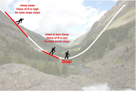
Gradient Descent - An Example

Imagine a person at the top of a mountain who wants to get to the bottom of the valley below the mountain through the fog (he cannot see clearly ahead and only can look around the point he's standing at)

He goes down the slope and takes large steps when the slope is steep and small steps when the slope is less steep.

He decides on his next position based on his current position and stops when he gets to the bottom of the valley, which was his goal.

Gradient Descent in action

Now, think of the valley as a cost function. The objective of GD is to minimize the cost function (by updating its parameter values). In this case, the minimum value would be 0.

What does a cost function look like?

J is the cost function, plotted along its parameter values. Notice the crests and troughs.

How we navigate the cost function via GD

Backward Propagation

What is Backward Propagation in NN?

• Backward propagation means moving in only one direction in a neural network, from output to input.
• Backward propagation is also called Backpropagation in short.

NOTE: Stochastic Gradient Descent (SGD) that the instructor sometimes mentions in the following video is just a type of Gradient Descent. Don't worry about its exact working.

Backpropagation Calculus (Optional)

If you like understanding things through Mathematics, this is for you! ????

Summarising the working of a NN

• A Neural Network passes data to the model via forward propagation.
• When it reaches the last(output) layer, it calculates loss on output.
• It then back propagates information about the loss/error, in reverse, through the network to the input layer so that it can alter the parameters/weights.
• Gradient Descent is calculated via Backpropagation and works to minimize this loss:
  • By calculating the gradient of loss function according to weights
  • Updating weights accordingly

Download the slides for this module from here.