Learning Objectives

• Spatial/ Translation Invariance
• Disadvantages of MLP
• Convolutional Neural Network
• Comparison of CNN and ANN/MLP architecture
• Deep Learning on Limited Data - Transfer learning, Data Augmentation
• Batch Normalization

Until now, you've worked with Multi-Layer Perceptrons(MLP).

MLPs are great for MNIST - a simpler, more straightforward dataset - but lag behind CNNs when it comes to real-world applications in computer vision, specifically image classification.

The concepts that make CNN so great are not complex but are very intuitive, logical, and easy to understand.

Spatial/Translation Invariance

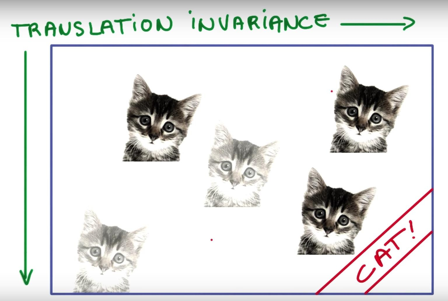
Spatial or Translation Invariance means that if an object occurs in any image it will be detected irrespective of its position.

A cat is still a cat regardless of whether it appears in the top half or the bottom half of the image.

Disadvantages of MLP

• Need to connect neurons in the hidden layer to ALL the neurons in the input layer
• No spatial information: Since we reshape the image from 2D to 1D, it doesn't understand the spatial structure of the image, i.e., it is not spatially invariant. For example, if a picture of a cat appears in the top left of the image in one picture and the bottom right of another picture, the MLP will try to correct itself and assume that a cat will always appear in this section of the image.

• And many, many parameters to be handled. MLPs use one perceptron for each input (e.g. pixel in an image, multiplied by 3 in RGB case). The amount of weights rapidly becomes unmanageable for large images. For a 224 x 224 pixel image with three color channels, there are around 150,000 weights that must be trained!

The Convolutional Neural Network

Convolutional Neural Networks are designed to be spatially invariant; they are not sensitive to the object's position in the picture. The cat can be anywhere in the image, and it'll still recognize it!

But what if the image doesn't just consist of a cat? What if there are more features? Will flipping the image confuse the CNN? No, a CNN will still work fine!

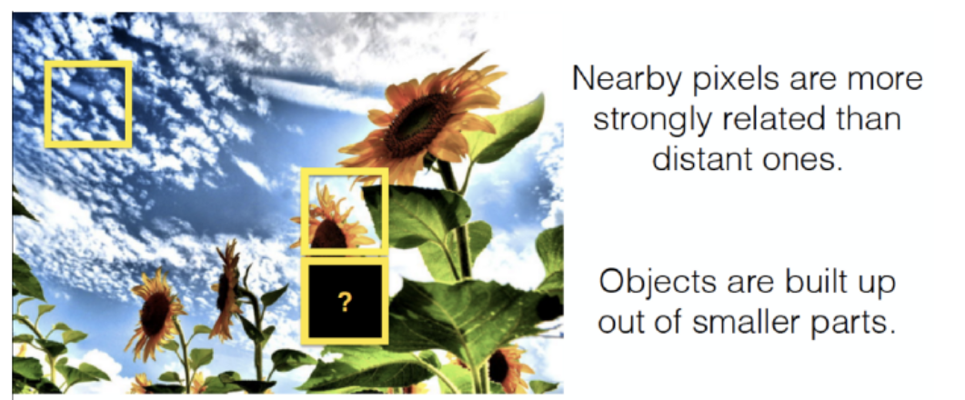
CNNs take advantage of the fact that nearby pixels are more strongly related than distant ones. So pixels around the sky will still be sky, and pixels near a sunflower have more chances of being a sunflower.

To teach an algorithm to recognize objects in images, we use a specific type of Artificial Neural Network: a Convolutional Neural Network (CNN). Their name stems from one of the most important operations in the network: convolution.

The word convolution refers to the filtering process that happens in this type of network. In literal terms, it is a mathematical operation that makes filtering possible.

Comparison of CNN and ANN/MLP

Regular Neural Networks:

• Transform an input by putting it through a series of hidden layers.
• Every layer is made up of a set of neurons, where each layer is fully connected to all neurons in the layer before.
• Finally, there is a last fully-connected layer — the output layer — that represents the predictions.

In CNNs :

• The layers are organized in 3 dimensions: width, height, and depth.
• The neurons in one layer do not connect to all the neurons in the next layer but only to a small region.

CNN Working

CNN Components

CNN's have two components:

1. The Hidden layers/Feature extraction part
   In this part, the network will perform a series of operations during which the features are detected. If you had a picture of a zebra, this is the part where the network would recognize its stripes, two ears, and four legs.
2. The Classification part
   This part assigns a probability of the object(e.g., The zebra) being in that image.

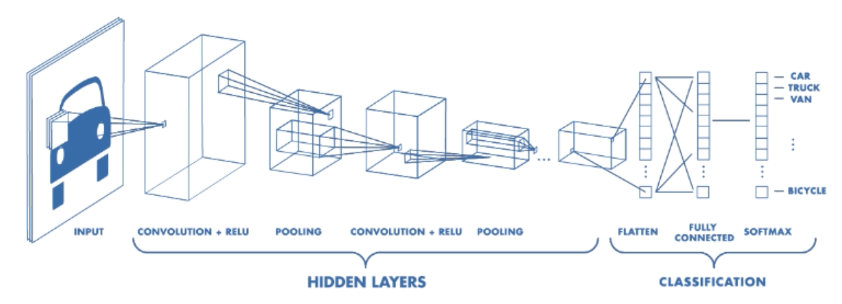
A basic CNN architecture

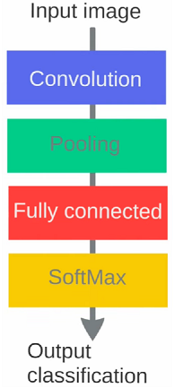
Below is the basic order of operations in a CNN. The Convolution and Pooling operations can occur multiple times in a CNN; the order will, however, remain the same. They'll always be succeeded by Fully Connected and Softmax/Sigmoid layers.

Basic Understanding of Filter, Stride & Convolution

This brilliantly explains how a kernel/filter makes convolution possible. For the people worried about how exactly one gets a particular size when applying a kernel on a matrix, this will solve your confusion.

What is zero Padding, and why is it even required?

Max Pooling

What do CNN layers learn?

• Each CNN layer learns filters of increasing complexity.
• The first layers learn basic feature detection filters: edges, corners, etc
• The middle layers learn filters that detect parts of objects. For faces, they might learn to respond to eyes, noses, etc
• The last layers have higher representations: they learn to recognize full objects, in different shapes and positions.

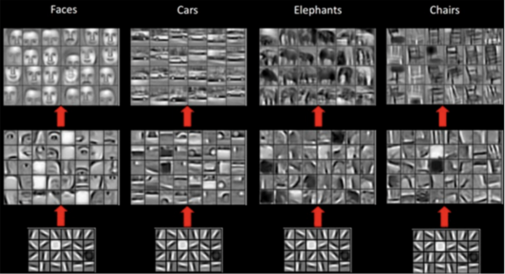
The earlier features of a ConvNet contain more generic features (e.g., edge detectors or color blob detectors), but later layers of the ConvNet become progressively more specific to the details of the classes contained in the original dataset.

How to use Deep Learning when you have limited data

The problem of Limited Data

"The analogy to deep learning is that the rocket engine is the deep learning models, and the fuel is the huge amounts of data we can feed to these algorithms." — Andrew Ng

There has been a recent surge in the popularity of Deep Learning, achieving state-of-the-art performance in various tasks like Language Translation, playing Strategy Games, and Self Driving Cars requiring millions of data points.

One common barrier to using deep learning to solve problems is the amount of data needed to train a model. The requirement for large data arises because of the number of parameters in the model that machines have to learn.

So what do you do when you cannot find the required data while working on a problem?

Transfer Learning to the Rescue!

"If Deep Learning is the holy grail and data is the gatekeeper, transfer learning is the key."

Transfer Learning

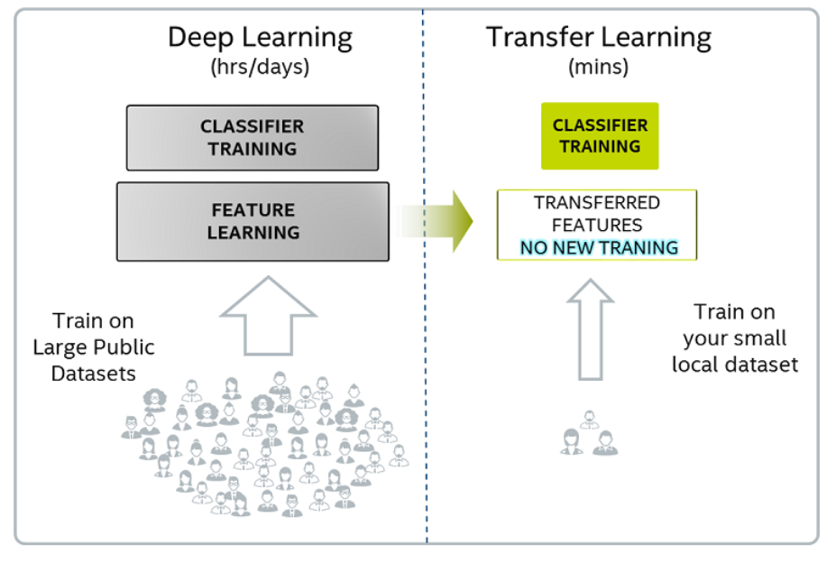
Transfer learning uses the knowledge gained while solving one problem and applying it to a different but related problem.

For example, knowledge gained while learning to recognize cars can be used to some extent to recognize trucks.

Pre-training

When we train a network on a large dataset(for example, ImageNet), we train all the neural network parameters, and therefore the model is learned. It may take hours on your GPU to train on such a large dataset. This model is known as a Pre-trained model.

Fine Tuning

We can give the new dataset to fine-tune the pre-trained CNN. Consider that the new dataset is almost similar to the original dataset used for pre-training. Since the new dataset is similar, the same weights can be used to extract the new dataset's features.

1. If the new dataset is very small, it's better to train only the final layers of the network to avoid overfitting, keeping all other layers fixed. So, remove the pre-trained network's final layers and add new ones. Retrain only the new layers.
2. If the new dataset is large, retrain the whole network with initial weights from the pre-trained model.

Another major advantage of using transfer learning is how well the model generalizes.

Larger models tend to overfit the data and don't work well when testing it out on unseen data. Since transfer learning allows the model to see different types of data, it learns the underlying rules of the world better.

You can look at this video if you're interested in learning how Transfer Learning is performed. It's a slightly advanced topic, so don't worry if you don't get it in the first go. Also, the instructor is using Keras but the same code will work with tf.Keras as well.

Data Augmentation

We need minor alterations to our existing dataset to get more data — minor changes such as flips, translations, or rotations. Our neural network would think these are distinct images anyway.

A convolutional neural network that can robustly classify objects even if its placed in different orientations is said to have the property called invariance. More specifically, a CNN can be invariant to translation, viewpoint, size, or illumination (Or a combination of the above).

This essentially is the premise of data augmentation. In a real-world scenario, we may have a dataset of images taken in a limited set of conditions. But, our target application may exist in various conditions, such as orientation, location, scale, brightness, etc. We account for these situations by training our neural network with additional synthetically modified data.

It is also one of the methods to prevent overfitting!

Your neural network is only as good as the data you feed it.

Performing augmentation can prevent your neural network from learning irrelevant patterns, essentially boosting overall performance.

Your model for detecting a butterfly should be able to find a butterfly in the image even if it is flying sidewards, right?

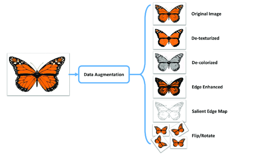
Popular Augmentation Techniques on images

1. Flip - horizontally/vertically
2. Rotation
3. Scale
4. Crop
5. Translation
6. Varying Color
7. Adding noise
8. Adjusting brightness

Apart from the above, many more augmentation techniques exist.

Where to perform Data Augmentation?

Data Augmentation is usually performed on Train Set and often Validation Set. This is because we want to increase the size and variety of data our model learns from.

However, Data Augmentation can also be performed on Test Set. It is not to make the test data bigger/more accurate but to make the input data from the test set resemble that of the input data from the training set so that we can feed it into the same net (e.g., same dimensions).

For example, in image cropping, we'd need to crop the test images too, so they are of a similar size as the training images.

How to perform Data Augmentation?

A Tensorflow Keras function called ImageDataGenerator helps in performing Data Augmentation techniques.

An ImageDataGenerator which performs augmentation might look like this:

1
2
3
4
5
6
7
8
9
train_datagen = ImageDataGenerator(
    rotation_range=20,
    width_shift_range=0.2,
    height_shift_range=0.2,
    shear_range=0.2,
    zoom_range=0.2,
    horizontal_flip=True
    vertical_flip=True,
    fill_mode='nearest')

Look at the variety of augmentation operations available!

Note: Apart from ImageDataGenerator, multiple other options exist for performing Data Augmentation.

Batch Normalization - Making models faster and more stable

Batch Normalization: What and Why?

Batch Normalization: How?

Applying Batch Normalization is as simple as adding a layer called BatchNormalization() after the convolution layer. It can be added to any Neural Network.

1
2
3
4
5
6
7
8
9
10
11
# Create the model model = Sequential()
model.add(Conv2D(32, kernel size=(3, 3), activation='relu', input shape=input_shape) 
model.add(BatchNormalization()) 
model.add(MaxPooling2D(pool_size=(2, 2)))
model.add(BatchNormalization())
model.add(Conv2D(64, kernel_size=(3, 3), activation='relu'))
model.add(BatchNormalization())
model.add(MaxPooling2D(pool_size=(2, 2)))
model.add(BatchNormalization()) model.add(Flatten()) model.add(Dense(256, activation='relu'))
model.add(BatchNormalization())
model.add(Dense(no_classes, activation='softmax')) 

Additional Material

A nice article throwing light on the variety of Data Augmentation techniques in practice:
https://towardsdatascience.com/exploring-image-data-augmentation-with-keras-and-tensorflow-a8162d89b844

Slide Download Link

You can download the slides for this module from here.

References

• https://towardsdatascience.com/what-is-transfer-learning-8b1a0fa42b4
• https://medium.com/nanonets/nanonets-how-to-use-deep-learning-when-you-have-limited-data-f68c0b512cab
• https://nanonets.com/blog/data-augmentation-how-to-use-deep-learning-when-you-have-limited-data-part-2/