Video Transcript

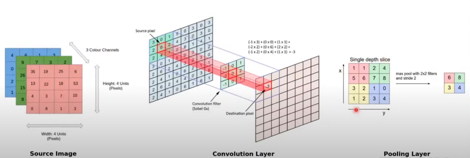
Now let's dive into the main layer components in a CNN. So as you can see, typically CNNs have a stack layered architecture. As you can see, it has multiple convolution blocks, pooling blocks, and so on. And inside each convolution block, it has multiple filters, as you can see here. And these filters are applied on the source image to give you what are known as feature maps. So convolution layer typically consists of several filters or kernels. And as we look into the TensorFlow API shortly, typically you specify the number of filters by a number, like let's say 16 filters, which means it will apply 16 specific kernels or filters on the source image and extract features. So that is where each filter or kernel is passed over the entire image in patches. And the filter is translated across the entire image. And we will see how this translation also occurs shortly what you need to know right now is this filter is passed through the entire image and translated across the entire image in patches. Let's say three cross three is an area of the image which we are focusing on. So nine pixels at a time. And what happens is the filter itself will be a specific dimension. Like let's say a three cross three filter with nine pixels. So what happens is a dot product is computed and the result is summed up to form one number per operation or per dot product. So in this way, these filters are applied on the source image and we end up with what are known as feature maps. And then what happens is we get a variety of feature maps based on the number of filters which we're applying. So let's say we have one source image and we apply 16 different convolution filters. So we will end up with 16 feature maps. The next step typically is to take in each of these feature maps and down sample them. So that is where we have what is called as the pooling layer which down samples the feature maps from the convolution layers. And typically there are various ways of down sampling. You can take the maximum of several pixels and basically output one maximum value pixel. You can take the average, you can take the sum and so on. But usually max pooling is used and we'll cover this also shortly as to why do we choose max pooling. And finally, as we discussed, every layer has a activation component to it where feature maps or pooled outputs are sent through nonlinear activations. And these nonlinear activations helps in introducing nonlinearity and trained via back propagation so that it just doesn't end up being a simple linear model. So now we will talk about the convolution pooling operations. So typically a source image can be a grayscale image which means it will be only a two dimensional image of a specific height and a width. And basically there will be various pixel values in the image. And the other aspect would be that if you are dealing with a colored image then there'll typically be three channels, red, green, and blue. And each of them will be a two dimensional matrix of pixel value. So basically this becomes like a three dimensional tensor. And considering a two dimensional image for simplicity right now, we'll go into how do you work on convolutions on a three dimensional image shortly. But considering you have a two dimensional image as you can see in the screen here, basically it is built of various pixel values at the end of the day. And each pixel has a very specific value depending on the gray level. And what happens is a convolution filter is basically a kernel. As you can see, this is a three cross three kernel with very specific values. And this is a Sobel kernel which means it helps in detecting edges. And what happens is this is basically translated across three cross three image patches one at a time. And then it computes the dot product and you end up getting a sum of this and that becomes your output pixel. So basically these convolution filters are translated across the image starting with 301262241. So this ends up giving you one final convolution output. And this is basically a feature map by the way. So this is your source image. This is your convolution filter and this is your feature map. So when you apply a three cross three convolution here you end up with one output. Similarly, then the filter is translated to this part of the image which means 015624410. Again, this is convolved with this filter and you end up with the next pixel value and so on and so forth. So basically it translates from left to right and then it goes down and again, left to right, so on and so forth. And you end up with one final feature map. And similarly, you apply different convolution filters to get different feature maps based on the number of filters which you specify in your convolution layer. And once you end up with a feature map like this then you can apply the downsampling or the pooling operation where let's say you want to apply a two cross two max pooling operation. What happens is it will take four pixels at a time and it will just output the max value. So in this way, you can see that from this feature map it has basically downsampled it to this final pooled output feature map. So in that way, you can reduce the dimensionality so that your training doesn't take forever and you don't end up overfitting on your data also. That's the advantage of using the pooling layer.

What are Convolutional Neural Networks?

Convolutional Neural Networks (ConvNets or CNNs) are a category of Neural Networks that have proven very effective in areas such as image recognition and classification. ConvNets have been successful in identifying faces, objects and traffic signs apart from powering vision in robots and self driving cars.

A Convolutional Neural Network (CNN) is comprised of one or more convolutional layers (often with a subsampling step) and then followed by one or more fully connected layers as in a standard multilayer neural network. The architecture of a CNN is designed to take advantage of the 2D structure of an input image (or other 2D input such as a speech signal). This is achieved with local connections and tied weights followed by some form of pooling which results in translation invariant features. Another benefit of CNNs is that they are easier to train and have many fewer parameters than fully connected networks with the same number of hidden units. In this article we will discuss the architecture of a CNN and the back propagation algorithm to compute the gradient with respect to the parameters of the model in order to use gradient based optimization.

Why Convolutions?

The spatial features of a 2D image are lost when it is flattened to a 1D vector input. Before feeding an image to the hidden layers of an MLP, we must flatten the image matrix to a 1D vector, as we saw in the mini project. This implies that all of the image's 2D information is discarded. Hence the need for convolutions.

Parameter Sharing

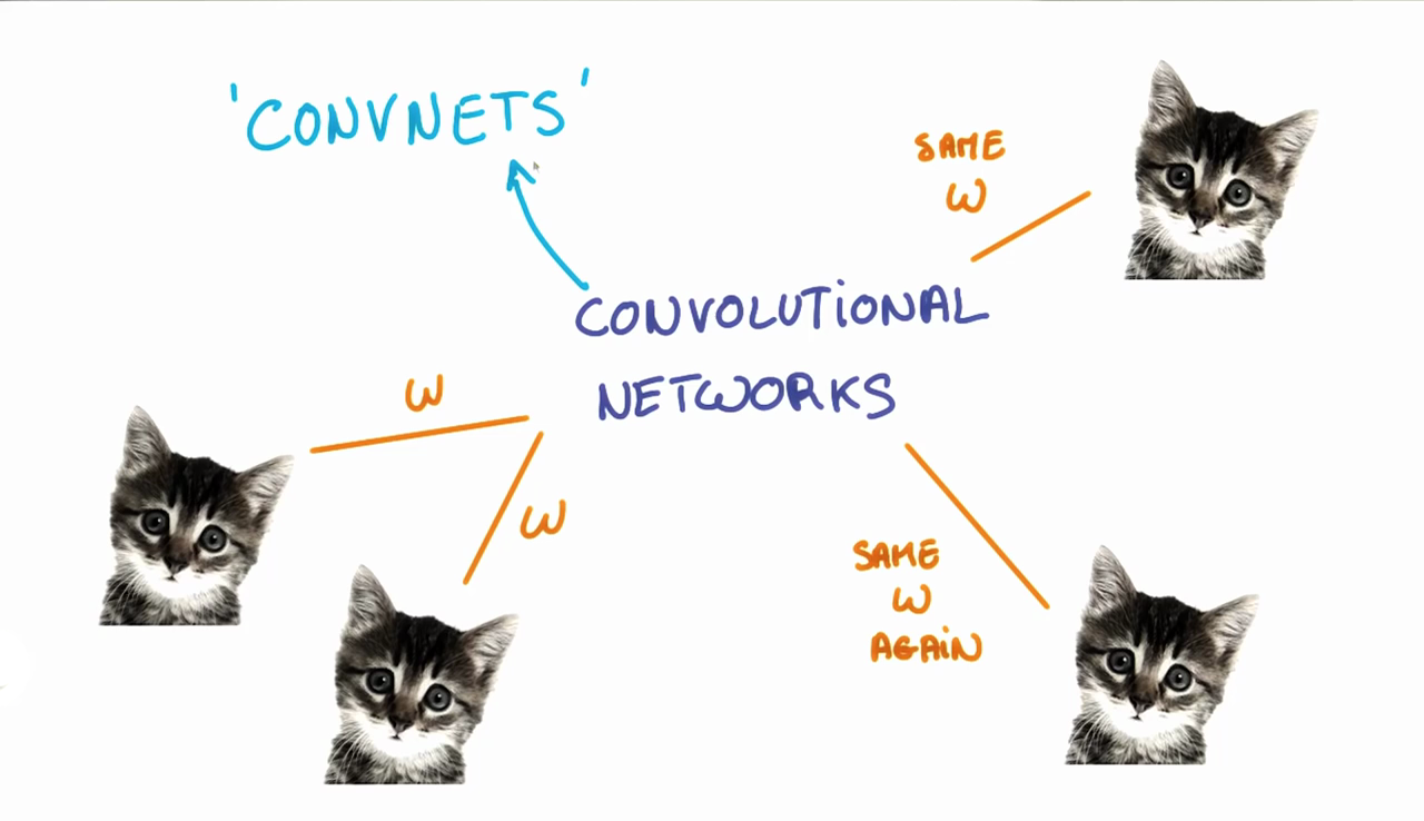
When we are trying to classify a picture of a cat, we don’t care where in the image a cat is. If it’s in the top left or the bottom right, it’s still a cat in our eyes. We would like our CNNs to also possess this ability known as translation invariance. How can we achieve this?

As we saw earlier, the classification of a given patch in an image is determined by the weights and biases corresponding to that patch.

If we want a cat that’s in the top left patch to be classified in the same way as a cat in the bottom right patch, we need the weights and biases corresponding to those patches to be the same, so that they are classified the same way.

This is exactly what we do in CNNs. The weights and biases we learn for a given output layer are shared across all patches in a given input layer. Note that as we increase the depth of our filter, the number of weights and biases we have to learn still increases, as the weights aren't shared across the output channels.

There’s an additional benefit to sharing our parameters. If we did not reuse the same weights across all patches, we would have to learn new parameters for every single patch and hidden layer neuron pair. This does not scale well, especially for higher fidelity images. Thus, sharing parameters not only helps us with translation invariance, but also gives us a smaller, more scalable model.

Major Components in a Convolutional Neural Network

• Input layer : All the input layer does is read the input image, so there are no parameters you could learn here.

• Convolutional layer: This layer is used to extract features.

• Pooling layer : This layer reduces number of weights and controls overfitting. No parameters are learned in this layer

• Flattening layer: This layer prepares the CNN layer output to be fed to a fully connected layer.

• Fully Connected layer : The fully connected layer is responsible for summing up all the detections made in the previous layers.They form the top layer of CNN Hierarchy

Convolutions

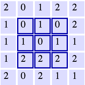
The above is an example of a convolution with a 3x3 filter and a stride of 1 being applied to data with a range of 0 to 1. The convolution for each 3x3 section is calculated against the weight,

It's good practice to remove the batches or features you want to skip from the data set rather than use stride to skip them. You can always set the first and last element to 1 in stride in order to use all batches and features.

Max Pooling

The above is an example of max pooling with a 2x2 filter and stride of 2. The left square is the input and the right square is the output. The four 2x2 colors in input represents each time the filter was applied to create the max on the right side. For example,

Padding

Let's say we have a

In an ideal world, we'd be able to maintain the same width and height across layers so that we can continue to add layers without worrying about the dimensionality shrinking and so that we have consistency. How might we achieve this? One way is to simple add a border of

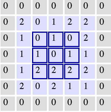
This would expand our original image to a